General usage

Input dataset

As a starting point, lets assume we have the following dataset, which was generated based on a harmonic model with some random component:

• NetCDF format

• One file per day

• Each file includes two variables “VAR1” and “VAR2”

• Half of the files are from the sensor “X1” and the other half from the sensor “X2”

• “X1” files have the data version “V1”, “X2” files have the data version “V5”

• The CRS of the data is the Equi7Grid projection of the European continent with a sampling of 24km

• The files are tiled into four adjacent tiles, each with a coverage of 600x600km

First, we need collect all file paths (around 3000) we want to put into our datacube. How to achieve this is up to you, but you can also use geopathfinder to conveniently gather files matching a certain file naming convention. Since our data is stored in one folder and we want to create a datacube of the whole dataset, we can use a simpler approach:

import os
import glob
import pprint
import numpy as np

ds_path = r"D:\data\code\yeoda\2022_08__docs\general_usage"
filepaths = glob.glob(os.path.join(ds_path, "*"))
np.array(filepaths)

array(['D:\\data\\code\\yeoda\\2022_08__docs\\general_usage\\DVAR_20000101T000000____E042N012T6_EU024KM_V1_X1.nc',
       'D:\\data\\code\\yeoda\\2022_08__docs\\general_usage\\DVAR_20000101T000000____E042N012T6_EU024KM_V5_X2.nc',
       'D:\\data\\code\\yeoda\\2022_08__docs\\general_usage\\DVAR_20000101T000000____E042N018T6_EU024KM_V1_X1.nc',
       ...,
       'D:\\data\\code\\yeoda\\2022_08__docs\\general_usage\\DVAR_20001230T000000____E048N012T6_EU024KM_V5_X2.nc',
       'D:\\data\\code\\yeoda\\2022_08__docs\\general_usage\\DVAR_20001230T000000____E048N018T6_EU024KM_V1_X1.nc',
       'D:\\data\\code\\yeoda\\2022_08__docs\\general_usage\\DVAR_20001230T000000____E048N018T6_EU024KM_V5_X2.nc'],
      dtype='<U98')

Datacube generation

As already brought up in the general package description, yeoda offers two basic datacube classes, DataCubeReader and DataCubeWriter. Both inherit from DataCube, which consists of the following essential components:

• File register: A data frame managing a stack/list of files containing the following columns:

  • “filepath”: Full system paths to the files.

  • stack_dimension (defaults to “layer_id”): Specifies an ID to which layer a file belongs to, e.g. a layer counter or a timestamp.

  • tile_dimension (defaults to “tile_id”): Tile name or ID to which tile a file belongs to.

• Mosaic geometry: An instance of MosaicGeometry (or a child class) managing the spatial properties or representing the actual mosaic/grid of the files

• Name of the tile (tile_dimension) and stack dimension (stack_dimension)

Initialising a DataCubeReader or DataCubeWriter object with a file register is most flexible, but can get tedious if one needs to create a complex data frame by hand. Therefore, both classes offer several class methods to quickly create a datacube instance covering most aspects when working with geospatial data. In the background, a datacube instance keeps a reference to a data format specific reader or writer class defined in veranda, which actually do all the magic in terms of data IO.

To be able to start playing around with a datacube object representing our prepared dataset, we can use the from_filepaths() method of DataCubeReader. This method tries to extract file-specific dimensions based on a certain filenaming convention (defined by the user or already pre-defined in geopathfinder) from the files and generates a file register, on-the-fly. Fortunately, the names of our files follow an existing file naming convention, namely YeodaFilename, which represents a generic file naming convention for EO data. If this would not have been the case, one can use geopathfinder’s SmartFilename class to create a new naming convention from scratch. According to this naming convention we can also define a set of dimension names we are interested in, i.e. the name of the stack/temporal and tile dimension, the variable, sensor, and data version dimension:

from yeoda.datacube import DataCubeReader
from geopathfinder.naming_conventions.yeoda_naming import YeodaFilename

dimensions = ["time", "tile_name", "var_name", "sensor_field", "data_version"]
dc_reader = DataCubeReader.from_filepaths(filepaths, fn_class=YeodaFilename, dimensions=dimensions,
                                          stack_dimension="time", tile_dimension="tile_name")
dc_reader

DataCubeReader -> NetCdfReader(time, MosaicGeometry):

                                               filepath   tile_name var_name  \
0     D:\data\code\yeoda\2022_08__docs\general_usage...  E042N012T6     DVAR
1     D:\data\code\yeoda\2022_08__docs\general_usage...  E042N012T6     DVAR
2     D:\data\code\yeoda\2022_08__docs\general_usage...  E042N018T6     DVAR
3     D:\data\code\yeoda\2022_08__docs\general_usage...  E042N018T6     DVAR
4     D:\data\code\yeoda\2022_08__docs\general_usage...  E048N012T6     DVAR
...                                                 ...         ...      ...
2915  D:\data\code\yeoda\2022_08__docs\general_usage...  E042N018T6     DVAR
2916  D:\data\code\yeoda\2022_08__docs\general_usage...  E048N012T6     DVAR
2917  D:\data\code\yeoda\2022_08__docs\general_usage...  E048N012T6     DVAR
2918  D:\data\code\yeoda\2022_08__docs\general_usage...  E048N018T6     DVAR
2919  D:\data\code\yeoda\2022_08__docs\general_usage...  E048N018T6     DVAR

     data_version sensor_field       time
0              V1           X1 2000-01-01
1              V5           X2 2000-01-01
2              V1           X1 2000-01-01
3              V5           X2 2000-01-01
4              V1           X1 2000-01-01
...           ...          ...        ...
2915           V5           X2 2000-12-30
2916           V1           X1 2000-12-30
2917           V5           X2 2000-12-30
2918           V1           X1 2000-12-30
2919           V5           X2 2000-12-30

[2920 rows x 6 columns]

What we can already directly see from the datacube’s print representation is the chosen reader class from veranda (i.e. NetCDFReader) with its dependent stack dimension (“time”) and associated mosaic class (MosaicGeometry). Additionally, the file register is shown, which reveals the decoded file naming parts of each file.

Datacube properties

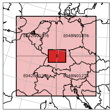
Our created datacube object has several properties to inspect. For instance, we can take a look at the mosaic to get an impression what spatial extent is covered by the dataset.

plot_extent = dc_reader.mosaic.outer_extent
extent_bfr = 200e3
plot_extent = [plot_extent[0] - extent_bfr, plot_extent[1] - extent_bfr,
               plot_extent[2] + extent_bfr, plot_extent[3] + extent_bfr]
dc_reader.mosaic.plot(label_tiles=True, extent=plot_extent)

<GeoAxesSubplot:>

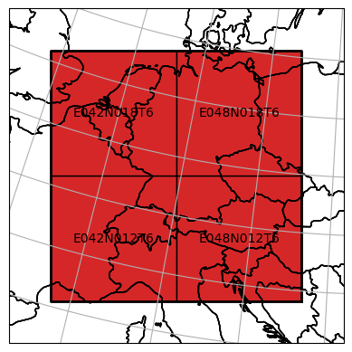
For further details about the mosaic, please take a look at geospade’s documentation.

It is also possible to directly access the file register,

dc_reader.file_register

	filepath	tile_name	var_name	data_version	sensor_field	time
0	D:\data\code\yeoda\2022_08__docs\general_usage...	E042N012T6	DVAR	V1	X1	2000-01-01
1	D:\data\code\yeoda\2022_08__docs\general_usage...	E042N012T6	DVAR	V5	X2	2000-01-01
2	D:\data\code\yeoda\2022_08__docs\general_usage...	E042N018T6	DVAR	V1	X1	2000-01-01
3	D:\data\code\yeoda\2022_08__docs\general_usage...	E042N018T6	DVAR	V5	X2	2000-01-01
4	D:\data\code\yeoda\2022_08__docs\general_usage...	E048N012T6	DVAR	V1	X1	2000-01-01
...	...	...	...	...	...	...
2915	D:\data\code\yeoda\2022_08__docs\general_usage...	E042N018T6	DVAR	V5	X2	2000-12-30
2916	D:\data\code\yeoda\2022_08__docs\general_usage...	E048N012T6	DVAR	V1	X1	2000-12-30
2917	D:\data\code\yeoda\2022_08__docs\general_usage...	E048N012T6	DVAR	V5	X2	2000-12-30
2918	D:\data\code\yeoda\2022_08__docs\general_usage...	E048N018T6	DVAR	V1	X1	2000-12-30
2919	D:\data\code\yeoda\2022_08__docs\general_usage...	E048N018T6	DVAR	V5	X2	2000-12-30

2920 rows × 6 columns

the number of tiles,

dc_reader.n_tiles

4

the file paths,

np.array(dc_reader.filepaths)

array(['D:\\data\\code\\yeoda\\2022_08__docs\\general_usage\\DVAR_20000503T000000____E048N012T6_EU024KM_V1_X1.nc',
       'D:\\data\\code\\yeoda\\2022_08__docs\\general_usage\\DVAR_20000826T000000____E048N012T6_EU024KM_V1_X1.nc',
       'D:\\data\\code\\yeoda\\2022_08__docs\\general_usage\\DVAR_20000625T000000____E042N012T6_EU024KM_V5_X2.nc',
       ...,
       'D:\\data\\code\\yeoda\\2022_08__docs\\general_usage\\DVAR_20001028T000000____E048N018T6_EU024KM_V5_X2.nc',
       'D:\\data\\code\\yeoda\\2022_08__docs\\general_usage\\DVAR_20000516T000000____E048N012T6_EU024KM_V5_X2.nc',
       'D:\\data\\code\\yeoda\\2022_08__docs\\general_usage\\DVAR_20000329T000000____E048N018T6_EU024KM_V5_X2.nc'],
      dtype='<U98')

the datacube dimensions,

dc_reader.dimensions

['tile_name', 'var_name', 'data_version', 'sensor_field', 'time']

and finally the actual (loaded) xarray data of the files on disk.

dc_reader.data_view

Since we did not read any data so far, this class attribute is none. The same holds true for a RasterGeometry instance associated with loaded data:

dc_reader.data_geom

To access actual coordinates along a certain dimension, a datacube instance supports indexing by means of the dimension name:

dc_reader['time']

0      2000-01-01
1      2000-01-01
2      2000-01-01
3      2000-01-01
4      2000-01-01
          ...
2915   2000-12-30
2916   2000-12-30
2917   2000-12-30
2918   2000-12-30
2919   2000-12-30
Name: time, Length: 2920, dtype: datetime64[ns]

In the next section you will learn how to select a subset of a datacube based on the file naming convention of the files. After performing such operations it is always a good idea to check the content of the file register. To quickly check if your selections led to an empty datacube, you can make use of another class property:

dc_reader.is_empty

False

File-specific selections

The most fundamental function for selecting a subset of the datacube is select_by_dimension(). It requires an expression, i.e. a function with one input argument (which will be replaced by a pd.Series containing the coordinate values along the specific dimension) linked to formula returning a boolean value if a row/coordinate should be selected or not, and the name of the dimension of interest.

Most datacube methods have a boolean key-word inplace defining if the current datacube instance should be modified or or a new one should be returned.

In the example below we are only interested in data from the sensor “X1”.

dc_sel = dc_reader.select_by_dimension(lambda s: s == "X1", name="sensor_field")
dc_sel.file_register

	filepath	tile_name	var_name	data_version	sensor_field	time
0	D:\data\code\yeoda\2022_08__docs\general_usage...	E042N012T6	DVAR	V1	X1	2000-01-01
2	D:\data\code\yeoda\2022_08__docs\general_usage...	E042N018T6	DVAR	V1	X1	2000-01-01
4	D:\data\code\yeoda\2022_08__docs\general_usage...	E048N012T6	DVAR	V1	X1	2000-01-01
6	D:\data\code\yeoda\2022_08__docs\general_usage...	E048N018T6	DVAR	V1	X1	2000-01-01
8	D:\data\code\yeoda\2022_08__docs\general_usage...	E042N012T6	DVAR	V1	X1	2000-01-02
...	...	...	...	...	...	...
2910	D:\data\code\yeoda\2022_08__docs\general_usage...	E048N018T6	DVAR	V1	X1	2000-12-29
2912	D:\data\code\yeoda\2022_08__docs\general_usage...	E042N012T6	DVAR	V1	X1	2000-12-30
2914	D:\data\code\yeoda\2022_08__docs\general_usage...	E042N018T6	DVAR	V1	X1	2000-12-30
2916	D:\data\code\yeoda\2022_08__docs\general_usage...	E048N012T6	DVAR	V1	X1	2000-12-30
2918	D:\data\code\yeoda\2022_08__docs\general_usage...	E048N018T6	DVAR	V1	X1	2000-12-30

1460 rows × 6 columns

More complex expressions are also possible, e.g. when selecting data/files within a specific date range.

import datetime
start_time, end_time = datetime.datetime(2000, 4, 1), datetime.datetime(2000, 5, 1)
dc_sel = dc_reader.select_by_dimension(lambda t: (t >= start_time) & (t <= end_time))
dc_sel.file_register

	filepath	tile_name	var_name	data_version	sensor_field	time
728	D:\data\code\yeoda\2022_08__docs\general_usage...	E042N012T6	DVAR	V1	X1	2000-04-01
729	D:\data\code\yeoda\2022_08__docs\general_usage...	E042N012T6	DVAR	V5	X2	2000-04-01
730	D:\data\code\yeoda\2022_08__docs\general_usage...	E042N018T6	DVAR	V1	X1	2000-04-01
731	D:\data\code\yeoda\2022_08__docs\general_usage...	E042N018T6	DVAR	V5	X2	2000-04-01
732	D:\data\code\yeoda\2022_08__docs\general_usage...	E048N012T6	DVAR	V1	X1	2000-04-01
...	...	...	...	...	...	...
971	D:\data\code\yeoda\2022_08__docs\general_usage...	E042N018T6	DVAR	V5	X2	2000-05-01
972	D:\data\code\yeoda\2022_08__docs\general_usage...	E048N012T6	DVAR	V1	X1	2000-05-01
973	D:\data\code\yeoda\2022_08__docs\general_usage...	E048N012T6	DVAR	V5	X2	2000-05-01
974	D:\data\code\yeoda\2022_08__docs\general_usage...	E048N018T6	DVAR	V1	X1	2000-05-01
975	D:\data\code\yeoda\2022_08__docs\general_usage...	E048N018T6	DVAR	V5	X2	2000-05-01

248 rows × 6 columns

Another way to filter certain file paths is select_files_with_pattern(), which applies a regex on the file names of the file register.

dc_sel = dc_reader.select_files_with_pattern(".*E042N018T6.*X2.*")
dc_sel.file_register

	filepath	tile_name	var_name	data_version	sensor_field	time
3	D:\data\code\yeoda\2022_08__docs\general_usage...	E042N018T6	DVAR	V5	X2	2000-01-01
11	D:\data\code\yeoda\2022_08__docs\general_usage...	E042N018T6	DVAR	V5	X2	2000-01-02
19	D:\data\code\yeoda\2022_08__docs\general_usage...	E042N018T6	DVAR	V5	X2	2000-01-03
27	D:\data\code\yeoda\2022_08__docs\general_usage...	E042N018T6	DVAR	V5	X2	2000-01-04
35	D:\data\code\yeoda\2022_08__docs\general_usage...	E042N018T6	DVAR	V5	X2	2000-01-05
...	...	...	...	...	...	...
2883	D:\data\code\yeoda\2022_08__docs\general_usage...	E042N018T6	DVAR	V5	X2	2000-12-26
2891	D:\data\code\yeoda\2022_08__docs\general_usage...	E042N018T6	DVAR	V5	X2	2000-12-27
2899	D:\data\code\yeoda\2022_08__docs\general_usage...	E042N018T6	DVAR	V5	X2	2000-12-28
2907	D:\data\code\yeoda\2022_08__docs\general_usage...	E042N018T6	DVAR	V5	X2	2000-12-29
2915	D:\data\code\yeoda\2022_08__docs\general_usage...	E042N018T6	DVAR	V5	X2	2000-12-30

365 rows × 6 columns

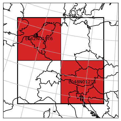
dc_sel = dc_reader.select_tiles(["E042N018T6", "E048N012T6"])
dc_sel.file_register

	filepath	tile_name	var_name	data_version	sensor_field	time
2	D:\data\code\yeoda\2022_08__docs\general_usage...	E042N018T6	DVAR	V1	X1	2000-01-01
3	D:\data\code\yeoda\2022_08__docs\general_usage...	E042N018T6	DVAR	V5	X2	2000-01-01
4	D:\data\code\yeoda\2022_08__docs\general_usage...	E048N012T6	DVAR	V1	X1	2000-01-01
5	D:\data\code\yeoda\2022_08__docs\general_usage...	E048N012T6	DVAR	V5	X2	2000-01-01
10	D:\data\code\yeoda\2022_08__docs\general_usage...	E042N018T6	DVAR	V1	X1	2000-01-02
...	...	...	...	...	...	...
2909	D:\data\code\yeoda\2022_08__docs\general_usage...	E048N012T6	DVAR	V5	X2	2000-12-29
2914	D:\data\code\yeoda\2022_08__docs\general_usage...	E042N018T6	DVAR	V1	X1	2000-12-30
2915	D:\data\code\yeoda\2022_08__docs\general_usage...	E042N018T6	DVAR	V5	X2	2000-12-30
2916	D:\data\code\yeoda\2022_08__docs\general_usage...	E048N012T6	DVAR	V1	X1	2000-12-30
2917	D:\data\code\yeoda\2022_08__docs\general_usage...	E048N012T6	DVAR	V5	X2	2000-12-30

1460 rows × 6 columns

Note that also the mosaic was filtered in the background:

dc_sel.mosaic.plot(label_tiles=True, extent=plot_extent)

<GeoAxesSubplot:>

Spatial selections

In the previous section we have seen how we can subset our datacube to select the data we actually want to work with. The last example introduced a first way how to perform a spatial selection of certain tiles, also affecting the properties of the mosaic.

Yet, one is most often interested in regions being much smaller than a tile or having a different spatial setting, e.g. a certain location, a bounding box, a non-rectangular region delineated by a polygon, or even an area crossing tile boundaries. yeoda’s datacube instances allow to perform all of those operations in a fluent manner, without touching any data. The following spatial selection methods expect the actual geometry of selection as positional arguments, and a SpatialRef instance as an optional key-word if the CRS of the geometry differs from the mosaic of the datacube.

Coordinate selection

If one is interested to retrieve a single time-series from the datacube, one can execute the following command.

from geospade.crs import SpatialRef

lat, lon = 48.21, 16.37 # centre of Vienna
sref = SpatialRef(4326)
dc_sel = dc_reader.select_xy(lat, lon, sref=sref)
dc_sel.file_register

	filepath	tile_name	var_name	data_version	sensor_field	time
4	D:\data\code\yeoda\2022_08__docs\general_usage...	E048N012T6	DVAR	V1	X1	2000-01-01
5	D:\data\code\yeoda\2022_08__docs\general_usage...	E048N012T6	DVAR	V5	X2	2000-01-01
12	D:\data\code\yeoda\2022_08__docs\general_usage...	E048N012T6	DVAR	V1	X1	2000-01-02
13	D:\data\code\yeoda\2022_08__docs\general_usage...	E048N012T6	DVAR	V5	X2	2000-01-02
20	D:\data\code\yeoda\2022_08__docs\general_usage...	E048N012T6	DVAR	V1	X1	2000-01-03
...	...	...	...	...	...	...
2901	D:\data\code\yeoda\2022_08__docs\general_usage...	E048N012T6	DVAR	V5	X2	2000-12-28
2908	D:\data\code\yeoda\2022_08__docs\general_usage...	E048N012T6	DVAR	V1	X1	2000-12-29
2909	D:\data\code\yeoda\2022_08__docs\general_usage...	E048N012T6	DVAR	V5	X2	2000-12-29
2916	D:\data\code\yeoda\2022_08__docs\general_usage...	E048N012T6	DVAR	V1	X1	2000-12-30
2917	D:\data\code\yeoda\2022_08__docs\general_usage...	E048N012T6	DVAR	V5	X2	2000-12-30

730 rows × 6 columns

As we can see, the file register only contains a reference to one tile, which covers our point of interest.

Bounding box selection

If we are interested in data covering a larger area, we can extend our single-point location to a bounding box.

bbox = [(48.22, 7.1), (49.36, 9,15)] # bounding box around Strasbourg and Karlsruhe
dc_sel = dc_reader.select_bbox(bbox, sref=sref)
dc_sel.file_register

	filepath	tile_name	var_name	data_version	sensor_field	time
0	D:\data\code\yeoda\2022_08__docs\general_usage...	E042N012T6	DVAR	V1	X1	2000-01-01
1	D:\data\code\yeoda\2022_08__docs\general_usage...	E042N012T6	DVAR	V5	X2	2000-01-01
2	D:\data\code\yeoda\2022_08__docs\general_usage...	E042N018T6	DVAR	V1	X1	2000-01-01
3	D:\data\code\yeoda\2022_08__docs\general_usage...	E042N018T6	DVAR	V5	X2	2000-01-01
8	D:\data\code\yeoda\2022_08__docs\general_usage...	E042N012T6	DVAR	V1	X1	2000-01-02
...	...	...	...	...	...	...
2907	D:\data\code\yeoda\2022_08__docs\general_usage...	E042N018T6	DVAR	V5	X2	2000-12-29
2912	D:\data\code\yeoda\2022_08__docs\general_usage...	E042N012T6	DVAR	V1	X1	2000-12-30
2913	D:\data\code\yeoda\2022_08__docs\general_usage...	E042N012T6	DVAR	V5	X2	2000-12-30
2914	D:\data\code\yeoda\2022_08__docs\general_usage...	E042N018T6	DVAR	V1	X1	2000-12-30
2915	D:\data\code\yeoda\2022_08__docs\general_usage...	E042N018T6	DVAR	V5	X2	2000-12-30

1460 rows × 6 columns

From the file register we can identify, that the bounding box crosses the border of the two western tiles.

Pixel window selection

Another possibility to read from a rectangular region of interest is to use the select_px_window() method, which accepts the upper-left row and column index as positional arguments and the extent of the pixel window with the keywords height and width.

The mosaic will only be sliced if it contains one tile to prevent ambiguities in terms of the definition of the pixel window. Otherwise the original datacube/mosaic will be returned.

dc_sel = dc_reader.select_tiles(["E042N018T6"])
dc_sel.select_px_window(10, 5, height=6, width=5, inplace=True)
dc_sel.mosaic.tiles[0].shape

(6, 5)

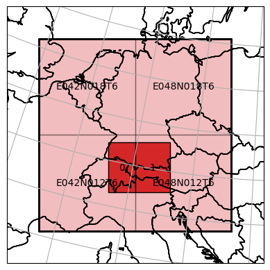
Polygon selection

As a final and most complex spatial selection example, one can also define a polygon (shapely or ogr polygon) as a region of interest.

from shapely.geometry import Polygon
polygon = Polygon(((4878945, 1835736),
                   (4927809, 1723051),
                   (4694460, 1730031),
                   (4776232, 1888589))) # given in native units; covers a region in southern Germany intersecting with all tiles
dc_roi = dc_reader.select_polygon(polygon)

ax = dc_reader.mosaic.plot(label_tiles=True, extent=plot_extent, alpha=0.3)
dc_roi.mosaic.plot(label_tiles=True, ax=ax, extent=plot_extent)
ax.plot(*polygon.exterior.coords.xy, color='b', alpha=0.7, label='Region of interest')

# this is how the actual data window would look like, i.e. the spatial coverage of the data read from disk
data_window_xs = dc_roi.mosaic.outer_extent[:1] * 2 + dc_roi.mosaic.outer_extent[2:3] * 2
data_window_ys = dc_roi.mosaic.outer_extent[1],  dc_roi.mosaic.outer_extent[3], dc_roi.mosaic.outer_extent[3], dc_roi.mosaic.outer_extent[1]
ax.plot(data_window_xs, data_window_ys, color='g', alpha=0.7, label='Data window')

ax.legend(ncol=2)

<matplotlib.legend.Legend at 0x2d1664a1670>

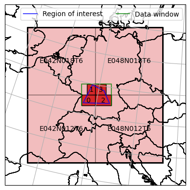
The plot above shows our region of interest defined as a polygon intersecting with all four tiles. The mosaic of dc_sel is now decoupled from the naming scheme of the original mosaic and contains four irregularly sliced tiles correspoding to the bounding box of the intersection figure of the polygon and each tile. Later on we will learn how to actually read the data from disk, whose outer pixel extent would be in alignment with the green bounding box.

Other datacube operations

In addition to the selection methods, a yeoda datacube has also a rich set of functions to manage and modify the datacube as needed.

Renaming a dimension

If one needs to work with a pre-defined naming convention, but is not happy with the name of a certain dimension/column of the file register, one can use the rename_dimensions() function mapping old to new dimension names.

dc_rnmd = dc_reader.rename_dimensions({'sensor_field': 'sensor'})
dc_rnmd.file_register

	filepath	tile_name	var_name	data_version	sensor	time
0	D:\data\code\yeoda\2022_08__docs\general_usage...	E042N012T6	DVAR	V1	X1	2000-01-01
1	D:\data\code\yeoda\2022_08__docs\general_usage...	E042N012T6	DVAR	V5	X2	2000-01-01
2	D:\data\code\yeoda\2022_08__docs\general_usage...	E042N018T6	DVAR	V1	X1	2000-01-01
3	D:\data\code\yeoda\2022_08__docs\general_usage...	E042N018T6	DVAR	V5	X2	2000-01-01
4	D:\data\code\yeoda\2022_08__docs\general_usage...	E048N012T6	DVAR	V1	X1	2000-01-01
...	...	...	...	...	...	...
2915	D:\data\code\yeoda\2022_08__docs\general_usage...	E042N018T6	DVAR	V5	X2	2000-12-30
2916	D:\data\code\yeoda\2022_08__docs\general_usage...	E048N012T6	DVAR	V1	X1	2000-12-30
2917	D:\data\code\yeoda\2022_08__docs\general_usage...	E048N012T6	DVAR	V5	X2	2000-12-30
2918	D:\data\code\yeoda\2022_08__docs\general_usage...	E048N018T6	DVAR	V1	X1	2000-12-30
2919	D:\data\code\yeoda\2022_08__docs\general_usage...	E048N018T6	DVAR	V5	X2	2000-12-30

2920 rows × 6 columns

Adding a new dimension

Sometimes it can be helpful to add one’s own dimension plus coordinate values to a datacube, e.g. file-specific properties like file size, quality flags, etc.

dim_values = np.random.rand(len(dc_reader))
dc_ext = dc_reader.add_dimension("value", dim_values)
dc_ext.file_register

	filepath	tile_name	var_name	data_version	sensor_field	time	value
0	D:\data\code\yeoda\2022_08__docs\general_usage...	E042N012T6	DVAR	V1	X1	2000-01-01	0.923070
1	D:\data\code\yeoda\2022_08__docs\general_usage...	E042N012T6	DVAR	V5	X2	2000-01-01	0.784735
2	D:\data\code\yeoda\2022_08__docs\general_usage...	E042N018T6	DVAR	V1	X1	2000-01-01	0.526505
3	D:\data\code\yeoda\2022_08__docs\general_usage...	E042N018T6	DVAR	V5	X2	2000-01-01	0.091429
4	D:\data\code\yeoda\2022_08__docs\general_usage...	E048N012T6	DVAR	V1	X1	2000-01-01	0.696233
...	...	...	...	...	...	...	...
2915	D:\data\code\yeoda\2022_08__docs\general_usage...	E042N018T6	DVAR	V5	X2	2000-12-30	0.983319
2916	D:\data\code\yeoda\2022_08__docs\general_usage...	E048N012T6	DVAR	V1	X1	2000-12-30	0.622559
2917	D:\data\code\yeoda\2022_08__docs\general_usage...	E048N012T6	DVAR	V5	X2	2000-12-30	0.416412
2918	D:\data\code\yeoda\2022_08__docs\general_usage...	E048N018T6	DVAR	V1	X1	2000-12-30	0.774230
2919	D:\data\code\yeoda\2022_08__docs\general_usage...	E048N018T6	DVAR	V5	X2	2000-12-30	0.375876

2920 rows × 7 columns

Sorting a dimension

As soon as you read data, each file will be accessed in the order given by file register. If you want to change this, i.e. to sort the files along a specific dimension, then you can use sort_by_dimension().

dc_srtd = dc_ext.sort_by_dimension('value', ascending=True)
dc_srtd.file_register

	filepath	tile_name	var_name	data_version	sensor_field	time	value
1732	D:\data\code\yeoda\2022_08__docs\general_usage...	E048N012T6	DVAR	V1	X1	2000-08-04	0.001752
219	D:\data\code\yeoda\2022_08__docs\general_usage...	E042N018T6	DVAR	V5	X2	2000-01-28	0.002179
2750	D:\data\code\yeoda\2022_08__docs\general_usage...	E048N018T6	DVAR	V1	X1	2000-12-09	0.002296
291	D:\data\code\yeoda\2022_08__docs\general_usage...	E042N018T6	DVAR	V5	X2	2000-02-06	0.002862
1913	D:\data\code\yeoda\2022_08__docs\general_usage...	E042N012T6	DVAR	V5	X2	2000-08-27	0.003018
...	...	...	...	...	...	...	...
2851	D:\data\code\yeoda\2022_08__docs\general_usage...	E042N018T6	DVAR	V5	X2	2000-12-22	0.998389
805	D:\data\code\yeoda\2022_08__docs\general_usage...	E048N012T6	DVAR	V5	X2	2000-04-10	0.998591
1309	D:\data\code\yeoda\2022_08__docs\general_usage...	E048N012T6	DVAR	V5	X2	2000-06-12	0.998791
2758	D:\data\code\yeoda\2022_08__docs\general_usage...	E048N018T6	DVAR	V1	X1	2000-12-10	0.998919
1349	D:\data\code\yeoda\2022_08__docs\general_usage...	E048N012T6	DVAR	V5	X2	2000-06-17	0.999556

2920 rows × 7 columns

Split up datacube by a dimension

Similar to the file-based selections, one can also use yeoda’s split functions to retrieve multiple datacubes from pre-defined coordinate intervals instead of writing multiple select statements. One function to do this is split_by_dimension.

dc_sensors = dc_reader.split_by_dimension([lambda s: s == 'X1', lambda s: s == 'X2'], name='sensor_field')
dc_sensors[1]

DataCubeReader -> NetCdfReader(time, MosaicGeometry):

                                               filepath   tile_name var_name  \
1     D:\data\code\yeoda\2022_08__docs\general_usage...  E042N012T6     DVAR
3     D:\data\code\yeoda\2022_08__docs\general_usage...  E042N018T6     DVAR
5     D:\data\code\yeoda\2022_08__docs\general_usage...  E048N012T6     DVAR
7     D:\data\code\yeoda\2022_08__docs\general_usage...  E048N018T6     DVAR
9     D:\data\code\yeoda\2022_08__docs\general_usage...  E042N012T6     DVAR
...                                                 ...         ...      ...
2911  D:\data\code\yeoda\2022_08__docs\general_usage...  E048N018T6     DVAR
2913  D:\data\code\yeoda\2022_08__docs\general_usage...  E042N012T6     DVAR
2915  D:\data\code\yeoda\2022_08__docs\general_usage...  E042N018T6     DVAR
2917  D:\data\code\yeoda\2022_08__docs\general_usage...  E048N012T6     DVAR
2919  D:\data\code\yeoda\2022_08__docs\general_usage...  E048N018T6     DVAR

     data_version sensor_field       time
1              V5           X2 2000-01-01
3              V5           X2 2000-01-01
5              V5           X2 2000-01-01
7              V5           X2 2000-01-01
9              V5           X2 2000-01-02
...           ...          ...        ...
2911           V5           X2 2000-12-29
2913           V5           X2 2000-12-30
2915           V5           X2 2000-12-30
2917           V5           X2 2000-12-30
2919           V5           X2 2000-12-30

[1460 rows x 6 columns]

Now we have two datacubes, one for each sensor.

Split up datacube temporally

Another handy function is split_by_temporal_freq(), which splits up the datacube into several smaller ones according to the specified temporal frequency identifier (see pandas DateOffset objects).

By default the stack dimension is assumed to be temporal. If not, you need to specify a different dimension with the key-word name.

dc_months = dc_reader.split_by_temporal_freq('M')
dc_months[1]

DataCubeReader -> NetCdfReader(time, MosaicGeometry):

                                              filepath   tile_name var_name  \
248  D:\data\code\yeoda\2022_08__docs\general_usage...  E042N012T6     DVAR
249  D:\data\code\yeoda\2022_08__docs\general_usage...  E042N012T6     DVAR
250  D:\data\code\yeoda\2022_08__docs\general_usage...  E042N018T6     DVAR
251  D:\data\code\yeoda\2022_08__docs\general_usage...  E042N018T6     DVAR
252  D:\data\code\yeoda\2022_08__docs\general_usage...  E048N012T6     DVAR
..                                                 ...         ...      ...
475  D:\data\code\yeoda\2022_08__docs\general_usage...  E042N018T6     DVAR
476  D:\data\code\yeoda\2022_08__docs\general_usage...  E048N012T6     DVAR
477  D:\data\code\yeoda\2022_08__docs\general_usage...  E048N012T6     DVAR
478  D:\data\code\yeoda\2022_08__docs\general_usage...  E048N018T6     DVAR
479  D:\data\code\yeoda\2022_08__docs\general_usage...  E048N018T6     DVAR

    data_version sensor_field       time
248           V1           X1 2000-02-01
249           V5           X2 2000-02-01
250           V1           X1 2000-02-01
251           V5           X2 2000-02-01
252           V1           X1 2000-02-01
..           ...          ...        ...
475           V5           X2 2000-02-29
476           V1           X1 2000-02-29
477           V5           X2 2000-02-29
478           V1           X1 2000-02-29
479           V5           X2 2000-02-29

[232 rows x 6 columns]

Copying a datacube

Sometimes it might be useful to create a (deep-)copy of a datacube object.

dc_cloned = dc_reader.clone()
dc_cloned.select_by_dimension(lambda v: v == 'V1', name='data_version', inplace=True)
print(f"Length of original datacube vs. cloned one: {len(dc_reader)} vs. {len(dc_cloned)}")

Length of original datacube vs. cloned one: 2920 vs. 1460

Multi-datacube operations

All aforementioned operations have only concerned one datacube object so far, but it is also possible to interact with two or more datacube instances.

Datacube union

If you have two datacube objects with a different set of dimensions or entries and want to unite (outer join) them, you can call unite. The following example demonstrates a union operation of two datacubes having different entries but the same dimensions.

dc_apr = dc_months[3]
dc_sept = dc_months[8]
dc_united = dc_apr.unite(dc_sept)
dc_united.file_register

	filepath	tile_name	var_name	data_version	sensor_field	time
0	D:\data\code\yeoda\2022_08__docs\general_usage...	E042N012T6	DVAR	V1	X1	2000-04-01
1	D:\data\code\yeoda\2022_08__docs\general_usage...	E042N012T6	DVAR	V5	X2	2000-04-01
2	D:\data\code\yeoda\2022_08__docs\general_usage...	E042N018T6	DVAR	V1	X1	2000-04-01
3	D:\data\code\yeoda\2022_08__docs\general_usage...	E042N018T6	DVAR	V5	X2	2000-04-01
4	D:\data\code\yeoda\2022_08__docs\general_usage...	E048N012T6	DVAR	V1	X1	2000-04-01
...	...	...	...	...	...	...
475	D:\data\code\yeoda\2022_08__docs\general_usage...	E042N018T6	DVAR	V5	X2	2000-09-30
476	D:\data\code\yeoda\2022_08__docs\general_usage...	E048N012T6	DVAR	V1	X1	2000-09-30
477	D:\data\code\yeoda\2022_08__docs\general_usage...	E048N012T6	DVAR	V5	X2	2000-09-30
478	D:\data\code\yeoda\2022_08__docs\general_usage...	E048N018T6	DVAR	V1	X1	2000-09-30
479	D:\data\code\yeoda\2022_08__docs\general_usage...	E048N018T6	DVAR	V5	X2	2000-09-30

480 rows × 6 columns

Another example would be if two datacubes differ in dimensions.

dc_1 = dc_reader.add_dimension('1', [1] * len(dc_reader))
dc_2 = dc_reader.add_dimension('2', [2] * len(dc_reader))
dc_united = dc_1.unite(dc_2)
dc_united.file_register

	filepath	tile_name	var_name	data_version	sensor_field	time	1	2
0	D:\data\code\yeoda\2022_08__docs\general_usage...	E042N012T6	DVAR	V1	X1	2000-01-01	1.0	NaN
1	D:\data\code\yeoda\2022_08__docs\general_usage...	E042N012T6	DVAR	V5	X2	2000-01-01	1.0	NaN
2	D:\data\code\yeoda\2022_08__docs\general_usage...	E042N018T6	DVAR	V1	X1	2000-01-01	1.0	NaN
3	D:\data\code\yeoda\2022_08__docs\general_usage...	E042N018T6	DVAR	V5	X2	2000-01-01	1.0	NaN
4	D:\data\code\yeoda\2022_08__docs\general_usage...	E048N012T6	DVAR	V1	X1	2000-01-01	1.0	NaN
...	...	...	...	...	...	...	...	...
5835	D:\data\code\yeoda\2022_08__docs\general_usage...	E042N018T6	DVAR	V5	X2	2000-12-30	NaN	2.0
5836	D:\data\code\yeoda\2022_08__docs\general_usage...	E048N012T6	DVAR	V1	X1	2000-12-30	NaN	2.0
5837	D:\data\code\yeoda\2022_08__docs\general_usage...	E048N012T6	DVAR	V5	X2	2000-12-30	NaN	2.0
5838	D:\data\code\yeoda\2022_08__docs\general_usage...	E048N018T6	DVAR	V1	X1	2000-12-30	NaN	2.0
5839	D:\data\code\yeoda\2022_08__docs\general_usage...	E048N018T6	DVAR	V5	X2	2000-12-30	NaN	2.0

5840 rows × 8 columns

Datacube intersection

Intersecting two datacubes works similarly, except that this time a inner join operation along the dimensions/columns of the file register takes place. As an optional argument, one can also define a specific dimension to operate the intersection along to perform an intersection also for the entries of the file register. The example below demonstrates an intersection to retrieve the common parts of two datacubes.

dc_apr_may = dc_months[3].unite(dc_months[4])
dc_may_jun = dc_months[4].unite(dc_months[5])
dc_intersct = dc_apr_may.intersect(dc_may_jun, on_dimension='time')
dc_intersct.file_register

	filepath	tile_name	var_name	data_version	sensor_field	time
0	D:\data\code\yeoda\2022_08__docs\general_usage...	E042N012T6	DVAR	V1	X1	2000-05-01
1	D:\data\code\yeoda\2022_08__docs\general_usage...	E042N012T6	DVAR	V5	X2	2000-05-01
2	D:\data\code\yeoda\2022_08__docs\general_usage...	E042N018T6	DVAR	V1	X1	2000-05-01
3	D:\data\code\yeoda\2022_08__docs\general_usage...	E042N018T6	DVAR	V5	X2	2000-05-01
4	D:\data\code\yeoda\2022_08__docs\general_usage...	E048N012T6	DVAR	V1	X1	2000-05-01
...	...	...	...	...	...	...
243	D:\data\code\yeoda\2022_08__docs\general_usage...	E042N018T6	DVAR	V5	X2	2000-05-31
244	D:\data\code\yeoda\2022_08__docs\general_usage...	E048N012T6	DVAR	V1	X1	2000-05-31
245	D:\data\code\yeoda\2022_08__docs\general_usage...	E048N012T6	DVAR	V5	X2	2000-05-31
246	D:\data\code\yeoda\2022_08__docs\general_usage...	E048N018T6	DVAR	V1	X1	2000-05-31
247	D:\data\code\yeoda\2022_08__docs\general_usage...	E048N018T6	DVAR	V5	X2	2000-05-31

248 rows × 6 columns

We can also take the two datacubes from before and intersect them to retrieve the original one.

dc_intersct = dc_1.intersect(dc_2)
dc_intersct.file_register

	filepath	tile_name	var_name	data_version	sensor_field	time
0	D:\data\code\yeoda\2022_08__docs\general_usage...	E042N012T6	DVAR	V1	X1	2000-01-01
1	D:\data\code\yeoda\2022_08__docs\general_usage...	E042N012T6	DVAR	V5	X2	2000-01-01
2	D:\data\code\yeoda\2022_08__docs\general_usage...	E042N018T6	DVAR	V1	X1	2000-01-01
3	D:\data\code\yeoda\2022_08__docs\general_usage...	E042N018T6	DVAR	V5	X2	2000-01-01
4	D:\data\code\yeoda\2022_08__docs\general_usage...	E048N012T6	DVAR	V1	X1	2000-01-01
...	...	...	...	...	...	...
2915	D:\data\code\yeoda\2022_08__docs\general_usage...	E042N018T6	DVAR	V5	X2	2000-12-30
2916	D:\data\code\yeoda\2022_08__docs\general_usage...	E048N012T6	DVAR	V1	X1	2000-12-30
2917	D:\data\code\yeoda\2022_08__docs\general_usage...	E048N012T6	DVAR	V5	X2	2000-12-30
2918	D:\data\code\yeoda\2022_08__docs\general_usage...	E048N018T6	DVAR	V1	X1	2000-12-30
2919	D:\data\code\yeoda\2022_08__docs\general_usage...	E048N018T6	DVAR	V5	X2	2000-12-30

2920 rows × 6 columns

Datacube alignment

As a last multi-datacube operation align_dimension allows to reduce or duplicate the number of entries in a datacube with respect to another datacube. However, it is only possible to resolve one-to-many or many-to-one relations with this method. The following example replicates the behaviour of the previously executed intersect operation. First, we need to ensure to only have unique entries along our dimension of interest.

dc_apr_tuni = dc_apr.select_tiles(["E042N012T6"])
_ = dc_apr_tuni.select_by_dimension(lambda s: s == 'X1', name='sensor_field', inplace=True)

Now we can try to align a large datacube to this smaller datacube along the temporal dimension by taking the many-to-one relation into account.

dc_1_apr = dc_1.align_dimension(dc_apr_tuni, 'time')
dc_1_apr.file_register

	filepath	tile_name	var_name	data_version	sensor_field	time	1
0	D:\data\code\yeoda\2022_08__docs\general_usage...	E042N012T6	DVAR	V1	X1	2000-04-01	1
1	D:\data\code\yeoda\2022_08__docs\general_usage...	E042N012T6	DVAR	V1	X1	2000-04-02	1
2	D:\data\code\yeoda\2022_08__docs\general_usage...	E042N012T6	DVAR	V1	X1	2000-04-03	1
3	D:\data\code\yeoda\2022_08__docs\general_usage...	E042N012T6	DVAR	V1	X1	2000-04-04	1
4	D:\data\code\yeoda\2022_08__docs\general_usage...	E042N012T6	DVAR	V1	X1	2000-04-05	1
5	D:\data\code\yeoda\2022_08__docs\general_usage...	E042N012T6	DVAR	V1	X1	2000-04-06	1
6	D:\data\code\yeoda\2022_08__docs\general_usage...	E042N012T6	DVAR	V1	X1	2000-04-07	1
7	D:\data\code\yeoda\2022_08__docs\general_usage...	E042N012T6	DVAR	V1	X1	2000-04-08	1
8	D:\data\code\yeoda\2022_08__docs\general_usage...	E042N012T6	DVAR	V1	X1	2000-04-09	1
9	D:\data\code\yeoda\2022_08__docs\general_usage...	E042N012T6	DVAR	V1	X1	2000-04-10	1
10	D:\data\code\yeoda\2022_08__docs\general_usage...	E042N012T6	DVAR	V1	X1	2000-04-11	1
11	D:\data\code\yeoda\2022_08__docs\general_usage...	E042N012T6	DVAR	V1	X1	2000-04-12	1
12	D:\data\code\yeoda\2022_08__docs\general_usage...	E042N012T6	DVAR	V1	X1	2000-04-13	1
13	D:\data\code\yeoda\2022_08__docs\general_usage...	E042N012T6	DVAR	V1	X1	2000-04-14	1
14	D:\data\code\yeoda\2022_08__docs\general_usage...	E042N012T6	DVAR	V1	X1	2000-04-15	1
15	D:\data\code\yeoda\2022_08__docs\general_usage...	E042N012T6	DVAR	V1	X1	2000-04-16	1
16	D:\data\code\yeoda\2022_08__docs\general_usage...	E042N012T6	DVAR	V1	X1	2000-04-17	1
17	D:\data\code\yeoda\2022_08__docs\general_usage...	E042N012T6	DVAR	V1	X1	2000-04-18	1
18	D:\data\code\yeoda\2022_08__docs\general_usage...	E042N012T6	DVAR	V1	X1	2000-04-19	1
19	D:\data\code\yeoda\2022_08__docs\general_usage...	E042N012T6	DVAR	V1	X1	2000-04-20	1
20	D:\data\code\yeoda\2022_08__docs\general_usage...	E042N012T6	DVAR	V1	X1	2000-04-21	1
21	D:\data\code\yeoda\2022_08__docs\general_usage...	E042N012T6	DVAR	V1	X1	2000-04-22	1
22	D:\data\code\yeoda\2022_08__docs\general_usage...	E042N012T6	DVAR	V1	X1	2000-04-23	1
23	D:\data\code\yeoda\2022_08__docs\general_usage...	E042N012T6	DVAR	V1	X1	2000-04-24	1
24	D:\data\code\yeoda\2022_08__docs\general_usage...	E042N012T6	DVAR	V1	X1	2000-04-25	1
25	D:\data\code\yeoda\2022_08__docs\general_usage...	E042N012T6	DVAR	V1	X1	2000-04-26	1
26	D:\data\code\yeoda\2022_08__docs\general_usage...	E042N012T6	DVAR	V1	X1	2000-04-27	1
27	D:\data\code\yeoda\2022_08__docs\general_usage...	E042N012T6	DVAR	V1	X1	2000-04-28	1
28	D:\data\code\yeoda\2022_08__docs\general_usage...	E042N012T6	DVAR	V1	X1	2000-04-29	1
29	D:\data\code\yeoda\2022_08__docs\general_usage...	E042N012T6	DVAR	V1	X1	2000-04-30	1

Another example would be if one wants to duplicate entries in a file register of a datacube so that both have the same length along the specified dimension. To demonstrate this, we can create a fake dataset, containing one file representing one observation of a sensor “X3” in a whole month.

fake_filepaths = [r"D:\data\code\yeoda\2022_08__docs\fake_data\DVAR_20000415T000000____E042N012T6_EU024KM_V1_X3.nc"]
dc_fake = DataCubeReader.from_filepaths(fake_filepaths, fn_class=YeodaFilename, dimensions=dimensions,
                                        stack_dimension="time", tile_dimension="tile_name")
dc_fake.file_register

	filepath	tile_name	var_name	data_version	sensor_field	time
0	D:\data\code\yeoda\2022_08__docs\fake_data\DVA...	E042N012T6	DVAR	V1	X3	2000-04-15

By calling align_dimension on this datacube with respect to a different datacube along a common dimension, we can duplicate the file register entries so that both datacubes match in length. In this case, we choose the “var_name” dimension as a common dimension, since its already available.

_ = dc_fake.align_dimension(dc_apr_tuni, "var_name", inplace=True)
dc_fake.file_register

	filepath	tile_name	var_name	data_version	sensor_field	time
0	D:\data\code\yeoda\2022_08__docs\fake_data\DVA...	E042N012T6	DVAR	V1	X3	2000-04-15
1	D:\data\code\yeoda\2022_08__docs\fake_data\DVA...	E042N012T6	DVAR	V1	X3	2000-04-15
2	D:\data\code\yeoda\2022_08__docs\fake_data\DVA...	E042N012T6	DVAR	V1	X3	2000-04-15
3	D:\data\code\yeoda\2022_08__docs\fake_data\DVA...	E042N012T6	DVAR	V1	X3	2000-04-15
4	D:\data\code\yeoda\2022_08__docs\fake_data\DVA...	E042N012T6	DVAR	V1	X3	2000-04-15
5	D:\data\code\yeoda\2022_08__docs\fake_data\DVA...	E042N012T6	DVAR	V1	X3	2000-04-15
6	D:\data\code\yeoda\2022_08__docs\fake_data\DVA...	E042N012T6	DVAR	V1	X3	2000-04-15
7	D:\data\code\yeoda\2022_08__docs\fake_data\DVA...	E042N012T6	DVAR	V1	X3	2000-04-15
8	D:\data\code\yeoda\2022_08__docs\fake_data\DVA...	E042N012T6	DVAR	V1	X3	2000-04-15
9	D:\data\code\yeoda\2022_08__docs\fake_data\DVA...	E042N012T6	DVAR	V1	X3	2000-04-15
10	D:\data\code\yeoda\2022_08__docs\fake_data\DVA...	E042N012T6	DVAR	V1	X3	2000-04-15
11	D:\data\code\yeoda\2022_08__docs\fake_data\DVA...	E042N012T6	DVAR	V1	X3	2000-04-15
12	D:\data\code\yeoda\2022_08__docs\fake_data\DVA...	E042N012T6	DVAR	V1	X3	2000-04-15
13	D:\data\code\yeoda\2022_08__docs\fake_data\DVA...	E042N012T6	DVAR	V1	X3	2000-04-15
14	D:\data\code\yeoda\2022_08__docs\fake_data\DVA...	E042N012T6	DVAR	V1	X3	2000-04-15
15	D:\data\code\yeoda\2022_08__docs\fake_data\DVA...	E042N012T6	DVAR	V1	X3	2000-04-15
16	D:\data\code\yeoda\2022_08__docs\fake_data\DVA...	E042N012T6	DVAR	V1	X3	2000-04-15
17	D:\data\code\yeoda\2022_08__docs\fake_data\DVA...	E042N012T6	DVAR	V1	X3	2000-04-15
18	D:\data\code\yeoda\2022_08__docs\fake_data\DVA...	E042N012T6	DVAR	V1	X3	2000-04-15
19	D:\data\code\yeoda\2022_08__docs\fake_data\DVA...	E042N012T6	DVAR	V1	X3	2000-04-15
20	D:\data\code\yeoda\2022_08__docs\fake_data\DVA...	E042N012T6	DVAR	V1	X3	2000-04-15
21	D:\data\code\yeoda\2022_08__docs\fake_data\DVA...	E042N012T6	DVAR	V1	X3	2000-04-15
22	D:\data\code\yeoda\2022_08__docs\fake_data\DVA...	E042N012T6	DVAR	V1	X3	2000-04-15
23	D:\data\code\yeoda\2022_08__docs\fake_data\DVA...	E042N012T6	DVAR	V1	X3	2000-04-15
24	D:\data\code\yeoda\2022_08__docs\fake_data\DVA...	E042N012T6	DVAR	V1	X3	2000-04-15
25	D:\data\code\yeoda\2022_08__docs\fake_data\DVA...	E042N012T6	DVAR	V1	X3	2000-04-15
26	D:\data\code\yeoda\2022_08__docs\fake_data\DVA...	E042N012T6	DVAR	V1	X3	2000-04-15
27	D:\data\code\yeoda\2022_08__docs\fake_data\DVA...	E042N012T6	DVAR	V1	X3	2000-04-15
28	D:\data\code\yeoda\2022_08__docs\fake_data\DVA...	E042N012T6	DVAR	V1	X3	2000-04-15
29	D:\data\code\yeoda\2022_08__docs\fake_data\DVA...	E042N012T6	DVAR	V1	X3	2000-04-15

Reading data

After you have selected the relevant files and spatial extent you want to read from, reading data from disk can be achieved with a single read() command. The arguments of the read function dependent on the actual data format of the dataset and are bound to the read() functions of the respective readers implemented in veranda. Therefore, it is recommended to look up the available arguments in the docstrings of the specific read() functions provided in veranda’s documentation.

Note that a DataCubeReader or DataCubeWriter instance keeps track of open file pointers. To ensure that everything is properly read from or written to disk either use the .close() function of a datacube instance or the with context when creating an instance.

As an example, we continue with the datacube generated from the more complex polygon selection, but split it up so that information from each sensor is separately loaded.

dc_roi_x1, dc_roi_x2 = dc_roi.split_by_dimension([lambda s: s == "X1", lambda s: s == "X2"], name='sensor_field')

Now we can read data stemming from sensor “X1” in a very slim manner.

dc_roi_x1.read()

This operation basically creates an internal xarray dataset, which can be viewed via the property data_view.

dc_roi_x1.data_view

<xarray.Dataset>
Dimensions:                (time: 365, y: 8, x: 11)
Coordinates:
  * time                   (time) datetime64[ns] 2000-01-01 ... 2000-12-30
  * y                      (y) float64 1.896e+06 1.872e+06 ... 1.728e+06
  * x                      (x) float64 4.68e+06 4.704e+06 ... 4.896e+06 4.92e+06
    azimuthal_equidistant  int32 0
Data variables:
    VAR1                   (time, y, x) float64 0.0 0.0 0.0 ... 2.174 2.224 2.21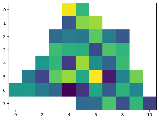
    VAR2                   (time, y, x) float64 0.0 0.0 0.0 ... 1.778 1.532

xarray.Dataset

• Dimensions:
  • time: 365
  • y: 8
  • x: 11
• Coordinates: (4)
  • time
    (time)
    datetime64[ns]
    2000-01-01 ... 2000-12-30

    array(['2000-01-01T00:00:00.000000000', '2000-01-02T00:00:00.000000000',
           '2000-01-03T00:00:00.000000000', ..., '2000-12-28T00:00:00.000000000',
           '2000-12-29T00:00:00.000000000', '2000-12-30T00:00:00.000000000'],
          dtype='datetime64[ns]')

  • y
    (y)
    float64
    1.896e+06 1.872e+06 ... 1.728e+06

    array([1896000., 1872000., 1848000., 1824000., 1800000., 1776000., 1752000.,
           1728000.])

  • x
    (x)
    float64
    4.68e+06 4.704e+06 ... 4.92e+06

    array([4680000., 4704000., 4728000., 4752000., 4776000., 4800000., 4824000.,
           4848000., 4872000., 4896000., 4920000.])

  • azimuthal_equidistant
    ()
    int32
    0

    crs_wkt :

    PROJCS["unknown",GEOGCS["unknown",DATUM["WGS_1984",SPHEROID["WGS 84",6378137,298.257223563,AUTHORITY["EPSG","7030"]],AUTHORITY["EPSG","6326"]],PRIMEM["Greenwich",0,AUTHORITY["EPSG","8901"]],UNIT["degree",0.0174532925199433,AUTHORITY["EPSG","9122"]]],PROJECTION["Azimuthal_Equidistant"],PARAMETER["latitude_of_center",53],PARAMETER["longitude_of_center",24],PARAMETER["false_easting",5837287.81977],PARAMETER["false_northing",2121415.69617],UNIT["metre",1,AUTHORITY["EPSG","9001"]],AXIS["Easting",EAST],AXIS["Northing",NORTH]]

    semi_major_axis :

    6378137.0

    semi_minor_axis :

    6356752.314245179

    inverse_flattening :

    298.257223563

    reference_ellipsoid_name :

    WGS 84

    longitude_of_prime_meridian :

    0.0

    prime_meridian_name :

    Greenwich

    geographic_crs_name :

    unknown

    horizontal_datum_name :

    World Geodetic System 1984

    projected_crs_name :

    unknown

    grid_mapping_name :

    azimuthal_equidistant

    latitude_of_projection_origin :

    53.0

    longitude_of_projection_origin :

    24.0

    false_easting :

    5837287.81977

    false_northing :

    2121415.69617

    spatial_ref :

    PROJCS["unknown",GEOGCS["unknown",DATUM["WGS_1984",SPHEROID["WGS 84",6378137,298.257223563,AUTHORITY["EPSG","7030"]],AUTHORITY["EPSG","6326"]],PRIMEM["Greenwich",0,AUTHORITY["EPSG","8901"]],UNIT["degree",0.0174532925199433,AUTHORITY["EPSG","9122"]]],PROJECTION["Azimuthal_Equidistant"],PARAMETER["latitude_of_center",53],PARAMETER["longitude_of_center",24],PARAMETER["false_easting",5837287.81977],PARAMETER["false_northing",2121415.69617],UNIT["metre",1,AUTHORITY["EPSG","9001"]],AXIS["Easting",EAST],AXIS["Northing",NORTH]]

    GeoTransform :

    0.0 4680000.0 24000.0 -24000.0 1896000.0 0.0

    array(0)

• Data variables: (2)
  • VAR1
    (time, y, x)
    float64
    0.0 0.0 0.0 ... 2.174 2.224 2.21

    _FillValue :

    0.0

    grid_mapping :

    azimuthal_equidistant

    array([[[0.        , 0.        , 0.        , ..., 0.        ,
             0.        , 0.        ],
            [0.        , 0.        , 0.        , ..., 0.        ,
             0.        , 0.        ],
            [0.        , 0.        , 0.        , ..., 2.26837642,
             0.        , 0.        ],
            ...,
            [0.        , 2.37986178, 2.27816473, ..., 2.27989214,
             2.21102074, 0.        ],
            [2.46620196, 2.22466741, 2.39449601, ..., 2.23331695,
             2.16583541, 0.        ],
            [0.        , 0.        , 0.        , ..., 2.22435886,
             2.35420984, 2.27922357]],
    
           [[0.        , 0.        , 0.        , ..., 0.        ,
             0.        , 0.        ],
            [0.        , 0.        , 0.        , ..., 0.        ,
             0.        , 0.        ],
            [0.        , 0.        , 0.        , ..., 2.28680691,
             0.        , 0.        ],
    ...
            [0.        , 2.10340733, 2.19454576, ..., 2.28804873,
             2.11951873, 0.        ],
            [2.32765573, 2.34199875, 2.12573666, ..., 2.12253719,
             2.33894847, 0.        ],
            [0.        , 0.        , 0.        , ..., 2.23080828,
             2.30818655, 2.5026298 ]],
    
           [[0.        , 0.        , 0.        , ..., 0.        ,
             0.        , 0.        ],
            [0.        , 0.        , 0.        , ..., 0.        ,
             0.        , 0.        ],
            [0.        , 0.        , 0.        , ..., 2.21430061,
             0.        , 0.        ],
            ...,
            [0.        , 2.20433995, 2.11086922, ..., 2.31363864,
             2.48553707, 0.        ],
            [2.17598537, 2.20018888, 2.20000903, ..., 2.21897424,
             2.35122964, 0.        ],
            [0.        , 0.        , 0.        , ..., 2.17360316,
             2.22411104, 2.20969408]]])

  • VAR2
    (time, y, x)
    float64
    0.0 0.0 0.0 ... 1.586 1.778 1.532

    _FillValue :

    0.0

    grid_mapping :

    azimuthal_equidistant

    array([[[0.        , 0.        , 0.        , ..., 0.        ,
             0.        , 0.        ],
            [0.        , 0.        , 0.        , ..., 0.        ,
             0.        , 0.        ],
            [0.        , 0.        , 0.        , ..., 1.53028419,
             0.        , 0.        ],
            ...,
            [0.        , 1.62100585, 1.75135119, ..., 1.66901398,
             1.45874145, 0.        ],
            [1.62711717, 1.67796973, 1.60052708, ..., 1.59234905,
             1.65863087, 0.        ],
            [0.        , 0.        , 0.        , ..., 1.653191  ,
             1.73863961, 1.62910462]],
    
           [[0.        , 0.        , 0.        , ..., 0.        ,
             0.        , 0.        ],
            [0.        , 0.        , 0.        , ..., 0.        ,
             0.        , 0.        ],
            [0.        , 0.        , 0.        , ..., 1.49396884,
             0.        , 0.        ],
    ...
            [0.        , 1.5666603 , 1.77004918, ..., 1.55027728,
             1.6409284 , 0.        ],
            [1.49715317, 1.57777091, 1.4981516 , ..., 1.65823371,
             1.56688149, 0.        ],
            [0.        , 0.        , 0.        , ..., 1.64501418,
             1.49258618, 1.57807059]],
    
           [[0.        , 0.        , 0.        , ..., 0.        ,
             0.        , 0.        ],
            [0.        , 0.        , 0.        , ..., 0.        ,
             0.        , 0.        ],
            [0.        , 0.        , 0.        , ..., 1.41738214,
             0.        , 0.        ],
            ...,
            [0.        , 1.50099737, 1.62356441, ..., 1.82927036,
             1.76017557, 0.        ],
            [1.68935618, 1.63471703, 1.67929967, ..., 1.37139682,
             1.49770883, 0.        ],
            [0.        , 0.        , 0.        , ..., 1.58551203,
             1.77826893, 1.53189952]]])

• Attributes: (0)

Lets look at one layer of the loaded dataset.

import matplotlib.pyplot as plt

data_layer = dc_roi_x1.data_view.sel({'time': [datetime.date(2000, 4, 1)]})
plt.imshow(data_layer['VAR1'].data[0, ...])

<matplotlib.image.AxesImage at 0x2d16648ac70>

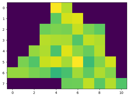
The pixel shape aligns well with the specified polygon, whereas the colour range does not show up as expected. This is because yeoda does not automatically set no data values to NaN, since this would require the data to be converted to float, which is not always desired in case of saving memory. In our case the no data value is 0, explaining the behaviour of the colourbar. To convert no data to NaN values, you can simply call apply_nan()

dc_roi_x1.apply_nan()

and recreate the plot.

data_layer = dc_roi_x1.data_view.sel({'time': [datetime.date(2000, 4, 1)]})
plt.imshow(data_layer['VAR1'].data[0, ...])

<matplotlib.image.AxesImage at 0x2d17f4f81f0>

Now every pixel outside the polygon is properly masked.

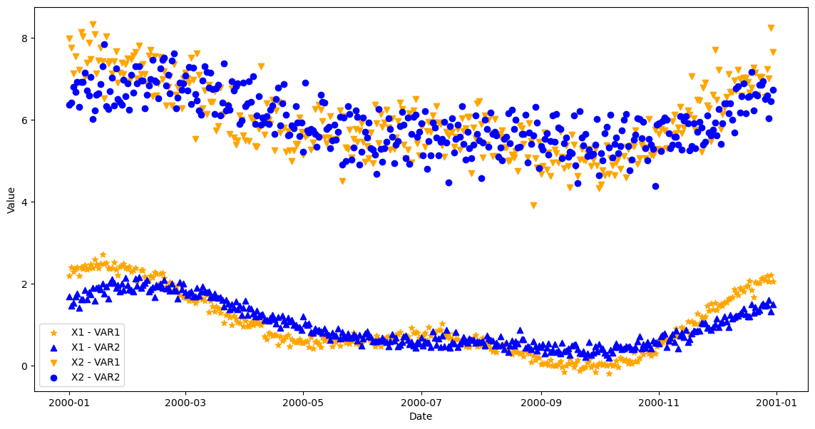
Another cool feature of yeoda’s datacube object is that you can apply select operations in space and along the stack dimension and the data is adapted accordingly. As long as you stay within the boundaries of the loaded dataset, there is no need to re-read data from disk, everything is done in memory. For instance we can load a single time series from both sensor datasets and plot it.

First, we still need to read the “X2” sensor data.

dc_roi_x2.read()

Then we define our point of interest

lat, lon = 49.16, 9.22 # city of Heilbronn in Germany
sref = SpatialRef(4326)
dc_x1_ts = dc_roi_x1.select_xy(lat, lon, sref=sref)
dc_x2_ts = dc_roi_x2.select_xy(lat, lon, sref=sref)
dc_x1_ts.data_view

<xarray.Dataset>
Dimensions:                (time: 365, y: 1, x: 1)
Coordinates:
  * time                   (time) datetime64[ns] 2000-01-01 ... 2000-12-30
  * y                      (y) float64 1.824e+06
  * x                      (x) float64 4.752e+06
    azimuthal_equidistant  int32 0
Data variables:
    VAR1                   (time, y, x) float64 2.189 2.407 ... 2.214 2.052
    VAR2                   (time, y, x) float64 1.681 1.454 1.528 ... 1.32 1.496

xarray.Dataset

• Dimensions:
  • time: 365
  • y: 1
  • x: 1
• Coordinates: (4)
  • time
    (time)
    datetime64[ns]
    2000-01-01 ... 2000-12-30

    array(['2000-01-01T00:00:00.000000000', '2000-01-02T00:00:00.000000000',
           '2000-01-03T00:00:00.000000000', ..., '2000-12-28T00:00:00.000000000',
           '2000-12-29T00:00:00.000000000', '2000-12-30T00:00:00.000000000'],
          dtype='datetime64[ns]')

  • y
    (y)
    float64
    1.824e+06

    array([1824000.])

  • x
    (x)
    float64
    4.752e+06

    array([4752000.])

  • azimuthal_equidistant
    ()
    int32
    0

    crs_wkt :

    PROJCS["unknown",GEOGCS["unknown",DATUM["WGS_1984",SPHEROID["WGS 84",6378137,298.257223563,AUTHORITY["EPSG","7030"]],AUTHORITY["EPSG","6326"]],PRIMEM["Greenwich",0,AUTHORITY["EPSG","8901"]],UNIT["degree",0.0174532925199433,AUTHORITY["EPSG","9122"]]],PROJECTION["Azimuthal_Equidistant"],PARAMETER["latitude_of_center",53],PARAMETER["longitude_of_center",24],PARAMETER["false_easting",5837287.81977],PARAMETER["false_northing",2121415.69617],UNIT["metre",1,AUTHORITY["EPSG","9001"]],AXIS["Easting",EAST],AXIS["Northing",NORTH]]

    semi_major_axis :

    6378137.0

    semi_minor_axis :

    6356752.314245179

    inverse_flattening :

    298.257223563

    reference_ellipsoid_name :

    WGS 84

    longitude_of_prime_meridian :

    0.0

    prime_meridian_name :

    Greenwich

    geographic_crs_name :

    unknown

    horizontal_datum_name :

    World Geodetic System 1984

    projected_crs_name :

    unknown

    grid_mapping_name :

    azimuthal_equidistant

    latitude_of_projection_origin :

    53.0

    longitude_of_projection_origin :

    24.0

    false_easting :

    5837287.81977

    false_northing :

    2121415.69617

    spatial_ref :

    PROJCS["unknown",GEOGCS["unknown",DATUM["WGS_1984",SPHEROID["WGS 84",6378137,298.257223563,AUTHORITY["EPSG","7030"]],AUTHORITY["EPSG","6326"]],PRIMEM["Greenwich",0,AUTHORITY["EPSG","8901"]],UNIT["degree",0.0174532925199433,AUTHORITY["EPSG","9122"]]],PROJECTION["Azimuthal_Equidistant"],PARAMETER["latitude_of_center",53],PARAMETER["longitude_of_center",24],PARAMETER["false_easting",5837287.81977],PARAMETER["false_northing",2121415.69617],UNIT["metre",1,AUTHORITY["EPSG","9001"]],AXIS["Easting",EAST],AXIS["Northing",NORTH]]

    GeoTransform :

    0.0 4680000.0 24000.0 -24000.0 1896000.0 0.0

    array(0)

• Data variables: (2)
  • VAR1
    (time, y, x)
    float64
    2.189 2.407 2.291 ... 2.214 2.052

    _FillValue :

    0.0

    grid_mapping :

    azimuthal_equidistant

    array([[[ 2.18935160e+00]],
    
           [[ 2.40732208e+00]],
    
           [[ 2.29120588e+00]],
    
           [[ 2.37401743e+00]],
    
           [[ 2.39870527e+00]],
    
           [[ 2.18574375e+00]],
    
           [[ 2.40818022e+00]],
    
           [[ 2.35823594e+00]],
    
           [[ 2.44747804e+00]],
    
           [[ 2.33966860e+00]],
    
    ...
    
           [[ 2.03491464e+00]],
    
           [[ 2.02333439e+00]],
    
           [[ 2.01213879e+00]],
    
           [[ 2.11875561e+00]],
    
           [[ 2.14041619e+00]],
    
           [[ 2.08642318e+00]],
    
           [[ 2.19576003e+00]],
    
           [[ 2.05305033e+00]],
    
           [[ 2.21432900e+00]],
    
           [[ 2.05241490e+00]]])

  • VAR2
    (time, y, x)
    float64
    1.681 1.454 1.528 ... 1.32 1.496

    _FillValue :

    0.0

    grid_mapping :

    azimuthal_equidistant

    array([[[1.68104528]],
    
           [[1.45427242]],
    
           [[1.52817816]],
    
           [[1.69412486]],
    
           [[1.75049424]],
    
           [[1.41451782]],
    
           [[1.61423654]],
    
           [[1.62465946]],
    
           [[1.84651059]],
    
           [[1.61309947]],
    
    ...
    
           [[1.41685731]],
    
           [[1.32008983]],
    
           [[1.34939001]],
    
           [[1.47834643]],
    
           [[1.52045934]],
    
           [[1.46577534]],
    
           [[1.47892782]],
    
           [[1.60424624]],
    
           [[1.32008364]],
    
           [[1.49600511]]])

• Attributes: (0)

and plot our extracted time series

ts = dc_x1_ts.data_view['time'].data
x1_var1_ts = dc_x1_ts.data_view['VAR1'].data.flatten()
x1_var2_ts = dc_x1_ts.data_view['VAR2'].data.flatten()
x2_var1_ts = dc_x2_ts.data_view['VAR1'].data.flatten()
x2_var2_ts = dc_x2_ts.data_view['VAR2'].data.flatten()
plt.figure(figsize=(14, 7))
plt.scatter(ts, x1_var1_ts, label='X1 - VAR1', color='orange', marker='*')
plt.scatter(ts, x1_var2_ts, label='X1 - VAR2', color='b', marker='^')
plt.scatter(ts, x2_var1_ts, label='X2 - VAR1', color='orange', marker='v')
plt.scatter(ts, x2_var2_ts, label='X2 - VAR2', color='b')
plt.ylabel('Value')
plt.xlabel('Date')
plt.legend()

<matplotlib.legend.Legend at 0x2d17f4ed790>

Writing data

yeoda’s DataCubeWriter class operates in the same manner as DataCubeReader, e.g. you can select and filter files, apply spatial subsetting, truncate data etc. Only the start and end point are different - instead of a from_filepaths() class method you can now use from_data() and instead of the read() function, one has the option to either use write() or export(). Similarly as from_filepaths(), from_data() automatically creates a file register based on a given file naming convention and some additional key-words assisting in interpreting coordinates of the xarray dataset. The key-word stack_group defines the relation between the stack coordinates and a group ID, i.e. in what portions along the stack dimension the data should be written.

The stack_group feature is only meaningful as long as the underlying data format supports to stack multiple files, e.g. NetCDF.

If stack_group is set, then you can assign new filename attributes to each group ID by using another optional argument fn_groups_map, which assigns filename fields to each group ID. In case the tile or stack dimension differ in naming from the chosen filenaming attributes, one can specify the mapping between dimension names and their corresponding filename entry with fn_map.

The spatial context is directly derived from the xarray dataset. If the dataset does not have any spatial reference information attached, one can create or use the mosaic of an existing datacube with the same spatial extent.

Data export

The first example represents the most simple case, i.e. one has read/created an xarray dataset, which should be written to disk as is. To do so, we first need to initialise a DataCubeWriter() instance by using the class method from_data(). Here, we can make use of the already available datacube dc_roi_x1 from the polygon region. We also need to specify the data location where to write the data to, which we choose to be temporary.

import tempfile

dst_dirpath = tempfile.mkdtemp()

Since we want to write one NetCDF stack to disk, we can create the following stacking arguments, mapping all time stamps of the xarray dataset to a group ID 0:

min_time, max_time = min(dc_roi_x1.data_view['time'].data), max(dc_roi_x1.data_view['time'].data)
stack_groups = {ts: 0 for ts in dc_roi_x1.data_view['time'].data}
fn_groups_map = {0: {'datetime_1': min_time, 'datetime_2': max_time}}

Static file name information can be set with def_fields.

def_fields = {'var_name': 'YVAR', 'sensor_field': 'X1'}

Now we have everything ready to initialise our DataCubeWriter object

from yeoda.datacube import DataCubeWriter

dc_writer_sngl_stack = DataCubeWriter.from_data(dc_roi_x1.data_view, dst_dirpath,
                                                fn_class=YeodaFilename, ext='.nc', def_fields=def_fields,
                                                stack_dimension='time', tile_dimension='tile_name',
                                                fn_map={'time': 'datetime_1'},
                                                stack_groups=stack_groups,
                                                fn_groups_map=fn_groups_map)
dc_writer_sngl_stack

DataCubeWriter -> NetCdfWriter(time, MosaicGeometry):

                                              filepath       time tile_name
0    C:\Users\cnavacch\AppData\Local\Temp\tmpjbzzes... 2000-01-01         0
1    C:\Users\cnavacch\AppData\Local\Temp\tmpjbzzes... 2000-01-02         0
2    C:\Users\cnavacch\AppData\Local\Temp\tmpjbzzes... 2000-01-03         0
3    C:\Users\cnavacch\AppData\Local\Temp\tmpjbzzes... 2000-01-04         0
4    C:\Users\cnavacch\AppData\Local\Temp\tmpjbzzes... 2000-01-05         0
..                                                 ...        ...       ...
360  C:\Users\cnavacch\AppData\Local\Temp\tmpjbzzes... 2000-12-26         0
361  C:\Users\cnavacch\AppData\Local\Temp\tmpjbzzes... 2000-12-27         0
362  C:\Users\cnavacch\AppData\Local\Temp\tmpjbzzes... 2000-12-28         0
363  C:\Users\cnavacch\AppData\Local\Temp\tmpjbzzes... 2000-12-29         0
364  C:\Users\cnavacch\AppData\Local\Temp\tmpjbzzes... 2000-12-30         0

[365 rows x 3 columns]

If we check the file paths, we can see that only one file path is stored in the file register.

dc_writer_sngl_stack.filepaths

['C:\\Users\\cnavacch\\AppData\\Local\\Temp\\tmpjbzzes9a\\YVAR_20000101T000000_20001230T000000___0___X1.nc']

A (default) mosaic was also generated automatically in compliance with the given data extent.

ax = dc_reader.mosaic.parent_root.plot(label_tiles=True, extent=plot_extent, alpha=0.3)
dc_writer_sngl_stack.mosaic.plot(label_tiles=True, ax=ax, extent=plot_extent)

<GeoAxesSubplot:>

Finally, one can export all internal data of the datacube to disk by calling export().

dc_writer_sngl_stack.export()

As already mentioned before, don’t forget to close all file pointers to actually flush the data to disk.

dc_writer_sngl_stack.close()

Taking a look at the destination, where we wrote our dataset to, reveals that the whole datacube has been written to disk as a single NetCDF file.

os.listdir(dst_dirpath)

['YVAR_20000101T000000_20001230T000000___0___X1.nc']

Data tiling

If one wants to be compliant with the original or even a new tiling scheme, one can initialise a DataCubeWriter object with the corresponding mosaic

dst_dirpath = tempfile.mkdtemp()
ori_mosaic = dc_reader.mosaic.parent_root
dc_writer_tld_stacks = DataCubeWriter.from_data(dc_roi_x1.data_view, dst_dirpath, mosaic=ori_mosaic,
                                                fn_class=YeodaFilename, ext='.nc', def_fields=def_fields,
                                                stack_dimension='time', tile_dimension='tile_name',
                                                fn_map={'time': 'datetime_1'},
                                                stack_groups=stack_groups,
                                                fn_groups_map=fn_groups_map)

and export the data, but this time with setting the key-word use_mosaic to True.

dc_writer_tld_stacks.export(use_mosaic=True)
dc_writer_tld_stacks.close()

Listing the content of the target directory shows that we have written a single NetCDF stack per tile, only containing the data within our region of interest.

os.listdir(dst_dirpath)

['YVAR_20000101T000000_20001230T000000___E042N012T6___X1.nc',
 'YVAR_20000101T000000_20001230T000000___E042N018T6___X1.nc',
 'YVAR_20000101T000000_20001230T000000___E048N012T6___X1.nc',
 'YVAR_20000101T000000_20001230T000000___E048N018T6___X1.nc']

Data streaming

Sometimes data is simply too large to be kept in memory or needs to be computed chunk wise. Therefore, a DataCubeWriter in yeoda provides the function write(), which works in the same manner as export(), but writes external data to disk, in correspondence with the mosaic of the datacube.

To demonstrate this, we can write the data stored in dc_roi_x1 to disk, but this time chunk by chunk. First, we reinitialise our datacube object by means of the file register of the existing datacube writer instance after removing the existing file.

os.remove(dc_writer_sngl_stack.filepaths[0])
dc_chunk_writer = DataCubeWriter(dc_writer_sngl_stack.mosaic, file_register=dc_writer_sngl_stack.file_register,
                                 stack_dimension='time', tile_dimension='tile_name',
                                 ext='.nc')

Then we extract two chunks from the existing data (first two and last two rows).

y_coords = dc_roi_x1.data_view['y'].data
chunk_1 = dc_roi_x1.data_view.sel({'y': y_coords[:2]})
chunk_2 = dc_roi_x1.data_view.sel({'y': y_coords[-2:]})

By using write(), we are able to write each chunk separately to disk, to the same single NetCDF file. Here, we need to activate use_mosaic again, since each chunk should be written inside the single-tile mosaic delineating the data extent we have loaded.

dc_chunk_writer.write(chunk_1, use_mosaic=True)
dc_chunk_writer.write(chunk_2, use_mosaic=True)
dc_chunk_writer.close()

If we read this NetCDF file again

dc_reader = DataCubeReader.from_filepaths(dc_chunk_writer.filepaths, fn_class=YeodaFilename, dimensions=dimensions,
                                          stack_dimension="layer_id", tile_dimension="tile_name")
dc_reader.read()
dc_reader.apply_nan()

dc_reader.data_view

<xarray.Dataset>
Dimensions:                (time: 365, y: 8, x: 11)
Coordinates:
  * time                   (time) datetime64[ns] 2000-01-01 ... 2000-12-30
  * y                      (y) float64 1.896e+06 1.872e+06 ... 1.728e+06
  * x                      (x) float64 4.68e+06 4.704e+06 ... 4.896e+06 4.92e+06
    azimuthal_equidistant  int32 0
Data variables:
    VAR1                   (time, y, x) float64 nan nan nan ... 2.174 2.224 2.21
    VAR2                   (time, y, x) float64 nan nan nan ... 1.778 1.532

xarray.Dataset

• Dimensions:
  • time: 365
  • y: 8
  • x: 11
• Coordinates: (4)
  • time
    (time)
    datetime64[ns]
    2000-01-01 ... 2000-12-30

    array(['2000-01-01T00:00:00.000000000', '2000-01-02T00:00:00.000000000',
           '2000-01-03T00:00:00.000000000', ..., '2000-12-28T00:00:00.000000000',
           '2000-12-29T00:00:00.000000000', '2000-12-30T00:00:00.000000000'],
          dtype='datetime64[ns]')

  • y
    (y)
    float64
    1.896e+06 1.872e+06 ... 1.728e+06

    array([1896000., 1872000., 1848000., 1824000., 1800000., 1776000., 1752000.,
           1728000.])

  • x
    (x)
    float64
    4.68e+06 4.704e+06 ... 4.92e+06

    array([4680000., 4704000., 4728000., 4752000., 4776000., 4800000., 4824000.,
           4848000., 4872000., 4896000., 4920000.])

  • azimuthal_equidistant
    ()
    int32
    0

    crs_wkt :

    PROJCS["unknown",GEOGCS["unknown",DATUM["WGS_1984",SPHEROID["WGS 84",6378137,298.257223563,AUTHORITY["EPSG","7030"]],AUTHORITY["EPSG","6326"]],PRIMEM["Greenwich",0,AUTHORITY["EPSG","8901"]],UNIT["degree",0.0174532925199433,AUTHORITY["EPSG","9122"]]],PROJECTION["Azimuthal_Equidistant"],PARAMETER["latitude_of_center",53],PARAMETER["longitude_of_center",24],PARAMETER["false_easting",5837287.81977],PARAMETER["false_northing",2121415.69617],UNIT["metre",1,AUTHORITY["EPSG","9001"]],AXIS["Easting",EAST],AXIS["Northing",NORTH]]

    semi_major_axis :

    6378137.0

    semi_minor_axis :

    6356752.314245179

    inverse_flattening :

    298.257223563

    reference_ellipsoid_name :

    WGS 84

    longitude_of_prime_meridian :

    0.0

    prime_meridian_name :

    Greenwich

    geographic_crs_name :

    unknown

    horizontal_datum_name :

    World Geodetic System 1984

    projected_crs_name :

    unknown

    grid_mapping_name :

    azimuthal_equidistant

    latitude_of_projection_origin :

    53.0

    longitude_of_projection_origin :

    24.0

    false_easting :

    5837287.81977

    false_northing :

    2121415.69617

    spatial_ref :

    PROJCS["unknown",GEOGCS["unknown",DATUM["WGS_1984",SPHEROID["WGS 84",6378137,298.257223563,AUTHORITY["EPSG","7030"]],AUTHORITY["EPSG","6326"]],PRIMEM["Greenwich",0,AUTHORITY["EPSG","8901"]],UNIT["degree",0.0174532925199433,AUTHORITY["EPSG","9122"]]],PROJECTION["Azimuthal_Equidistant"],PARAMETER["latitude_of_center",53],PARAMETER["longitude_of_center",24],PARAMETER["false_easting",5837287.81977],PARAMETER["false_northing",2121415.69617],UNIT["metre",1,AUTHORITY["EPSG","9001"]],AXIS["Easting",EAST],AXIS["Northing",NORTH]]

    GeoTransform :

    0.0 4680000.0 24000.0 -24000.0 1896000.0 0.0

    array(0)

• Data variables: (2)
  • VAR1
    (time, y, x)
    float64
    nan nan nan ... 2.174 2.224 2.21

    _FillValue :

    0.0

    grid_mapping :

    azimuthal_equidistant

    array([[[       nan,        nan,        nan, ...,        nan,
                    nan,        nan],
            [       nan,        nan,        nan, ...,        nan,
                    nan,        nan],
            [       nan,        nan,        nan, ...,        nan,
                    nan,        nan],
            ...,
            [       nan,        nan,        nan, ...,        nan,
                    nan,        nan],
            [2.46620196, 2.22466741, 2.39449601, ..., 2.23331695,
             2.16583541,        nan],
            [       nan,        nan,        nan, ..., 2.22435886,
             2.35420984, 2.27922357]],
    
           [[       nan,        nan,        nan, ...,        nan,
                    nan,        nan],
            [       nan,        nan,        nan, ...,        nan,
                    nan,        nan],
            [       nan,        nan,        nan, ...,        nan,
                    nan,        nan],
    ...
            [       nan,        nan,        nan, ...,        nan,
                    nan,        nan],
            [2.32765573, 2.34199875, 2.12573666, ..., 2.12253719,
             2.33894847,        nan],
            [       nan,        nan,        nan, ..., 2.23080828,
             2.30818655, 2.5026298 ]],
    
           [[       nan,        nan,        nan, ...,        nan,
                    nan,        nan],
            [       nan,        nan,        nan, ...,        nan,
                    nan,        nan],
            [       nan,        nan,        nan, ...,        nan,
                    nan,        nan],
            ...,
            [       nan,        nan,        nan, ...,        nan,
                    nan,        nan],
            [2.17598537, 2.20018888, 2.20000903, ..., 2.21897424,
             2.35122964,        nan],
            [       nan,        nan,        nan, ..., 2.17360316,
             2.22411104, 2.20969408]]])

  • VAR2
    (time, y, x)
    float64
    nan nan nan ... 1.586 1.778 1.532

    _FillValue :

    0.0

    grid_mapping :

    azimuthal_equidistant

    array([[[       nan,        nan,        nan, ...,        nan,
                    nan,        nan],
            [       nan,        nan,        nan, ...,        nan,
                    nan,        nan],
            [       nan,        nan,        nan, ...,        nan,
                    nan,        nan],
            ...,
            [       nan,        nan,        nan, ...,        nan,
                    nan,        nan],
            [1.62711717, 1.67796973, 1.60052708, ..., 1.59234905,
             1.65863087,        nan],
            [       nan,        nan,        nan, ..., 1.653191  ,
             1.73863961, 1.62910462]],
    
           [[       nan,        nan,        nan, ...,        nan,
                    nan,        nan],
            [       nan,        nan,        nan, ...,        nan,
                    nan,        nan],
            [       nan,        nan,        nan, ...,        nan,
                    nan,        nan],
    ...
            [       nan,        nan,        nan, ...,        nan,
                    nan,        nan],
            [1.49715317, 1.57777091, 1.4981516 , ..., 1.65823371,
             1.56688149,        nan],
            [       nan,        nan,        nan, ..., 1.64501418,
             1.49258618, 1.57807059]],
    
           [[       nan,        nan,        nan, ...,        nan,
                    nan,        nan],
            [       nan,        nan,        nan, ...,        nan,
                    nan,        nan],
            [       nan,        nan,        nan, ...,        nan,
                    nan,        nan],
            ...,
            [       nan,        nan,        nan, ...,        nan,
                    nan,        nan],
            [1.68935618, 1.63471703, 1.67929967, ..., 1.37139682,
             1.49770883,        nan],
            [       nan,        nan,        nan, ..., 1.58551203,
             1.77826893, 1.53189952]]])

• Attributes: (0)

and take a look at the same layer as before

data_layer = dc_reader.data_view.sel({'time': [datetime.date(2000, 4, 1)]})
plt.imshow(data_layer['VAR1'].data[0, ...])

<matplotlib.image.AxesImage at 0x2d14074a0a0>

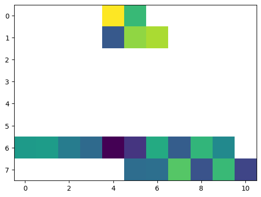
reveals that only the two data chunks have been written to disk.

Data format conversion

Finally, yeoda also allows to switch fluently between different data formats. For instance, we can convert a subset of the NetCDF files representing our original input dataset to multi-band GeoTIFF files. To do so, we reinitialise the datacube reader,

dc_reader_nc = DataCubeReader.from_filepaths(filepaths, fn_class=YeodaFilename, dimensions=dimensions,
                                             stack_dimension="time", tile_dimension="tile_name")

select a sensor,

dc_reader_nc.select_by_dimension(lambda s: s == "X2", name="sensor_field", inplace=True)

DataCubeReader -> NetCdfReader(time, MosaicGeometry):

                                               filepath   tile_name var_name  \
1     D:\data\code\yeoda\2022_08__docs\general_usage...  E042N012T6     DVAR
3     D:\data\code\yeoda\2022_08__docs\general_usage...  E042N018T6     DVAR
5     D:\data\code\yeoda\2022_08__docs\general_usage...  E048N012T6     DVAR
7     D:\data\code\yeoda\2022_08__docs\general_usage...  E048N018T6     DVAR
9     D:\data\code\yeoda\2022_08__docs\general_usage...  E042N012T6     DVAR
...                                                 ...         ...      ...
2911  D:\data\code\yeoda\2022_08__docs\general_usage...  E048N018T6     DVAR
2913  D:\data\code\yeoda\2022_08__docs\general_usage...  E042N012T6     DVAR
2915  D:\data\code\yeoda\2022_08__docs\general_usage...  E042N018T6     DVAR
2917  D:\data\code\yeoda\2022_08__docs\general_usage...  E048N012T6     DVAR
2919  D:\data\code\yeoda\2022_08__docs\general_usage...  E048N018T6     DVAR

     data_version sensor_field       time
1              V5           X2 2000-01-01
3              V5           X2 2000-01-01
5              V5           X2 2000-01-01
7              V5           X2 2000-01-01
9              V5           X2 2000-01-02
...           ...          ...        ...
2911           V5           X2 2000-12-29
2913           V5           X2 2000-12-30
2915           V5           X2 2000-12-30
2917           V5           X2 2000-12-30
2919           V5           X2 2000-12-30

[1460 rows x 6 columns]

a time frame,

start_time, end_time = datetime.datetime(2000, 11, 1),  datetime.datetime(2000, 12, 1)
dc_reader_nc.select_by_dimension(lambda t: (t >= start_time) & (t < end_time), name="time", inplace=True)

DataCubeReader -> NetCdfReader(time, MosaicGeometry):

                                               filepath   tile_name var_name  \
2441  D:\data\code\yeoda\2022_08__docs\general_usage...  E042N012T6     DVAR
2443  D:\data\code\yeoda\2022_08__docs\general_usage...  E042N018T6     DVAR
2445  D:\data\code\yeoda\2022_08__docs\general_usage...  E048N012T6     DVAR
2447  D:\data\code\yeoda\2022_08__docs\general_usage...  E048N018T6     DVAR
2449  D:\data\code\yeoda\2022_08__docs\general_usage...  E042N012T6     DVAR
...                                                 ...         ...      ...
2671  D:\data\code\yeoda\2022_08__docs\general_usage...  E048N018T6     DVAR
2673  D:\data\code\yeoda\2022_08__docs\general_usage...  E042N012T6     DVAR
2675  D:\data\code\yeoda\2022_08__docs\general_usage...  E042N018T6     DVAR
2677  D:\data\code\yeoda\2022_08__docs\general_usage...  E048N012T6     DVAR
2679  D:\data\code\yeoda\2022_08__docs\general_usage...  E048N018T6     DVAR

     data_version sensor_field       time
2441           V5           X2 2000-11-01
2443           V5           X2 2000-11-01
2445           V5           X2 2000-11-01
2447           V5           X2 2000-11-01
2449           V5           X2 2000-11-02
...           ...          ...        ...
2671           V5           X2 2000-11-29
2673           V5           X2 2000-11-30
2675           V5           X2 2000-11-30
2677           V5           X2 2000-11-30
2679           V5           X2 2000-11-30

[120 rows x 6 columns]

and a spatial subsetting with a bounding box intersecting on common tile border.

bbox = [(4649919, 1442955), (5006606, 1748127)]
_ = dc_reader_nc.select_bbox(bbox, inplace=True)

ax = dc_reader_nc.mosaic.parent_root.plot(label_tiles=True, extent=plot_extent, alpha=0.3)
dc_reader_nc.mosaic.plot(label_tiles=True, ax=ax, extent=plot_extent)

<GeoAxesSubplot:>

After reading the data

dc_reader_nc.read()
dc_reader_nc.data_view

<xarray.Dataset>
Dimensions:                (time: 30, y: 13, x: 16)
Coordinates:
  * time                   (time) datetime64[ns] 2000-11-01 ... 2000-11-30
  * y                      (y) float64 1.752e+06 1.728e+06 ... 1.464e+06
  * x                      (x) float64 4.632e+06 4.656e+06 ... 4.992e+06
    azimuthal_equidistant  int32 0
Data variables:
    VAR1                   (time, y, x) float64 5.657 5.406 ... 6.203 6.406
    VAR2                   (time, y, x) float64 5.505 5.846 ... 5.574 6.236

xarray.Dataset

• Dimensions:
  • time: 30
  • y: 13
  • x: 16
• Coordinates: (4)
  • time
    (time)
    datetime64[ns]
    2000-11-01 ... 2000-11-30

    array(['2000-11-01T00:00:00.000000000', '2000-11-02T00:00:00.000000000',
           '2000-11-03T00:00:00.000000000', '2000-11-04T00:00:00.000000000',
           '2000-11-05T00:00:00.000000000', '2000-11-06T00:00:00.000000000',
           '2000-11-07T00:00:00.000000000', '2000-11-08T00:00:00.000000000',
           '2000-11-09T00:00:00.000000000', '2000-11-10T00:00:00.000000000',
           '2000-11-11T00:00:00.000000000', '2000-11-12T00:00:00.000000000',
           '2000-11-13T00:00:00.000000000', '2000-11-14T00:00:00.000000000',
           '2000-11-15T00:00:00.000000000', '2000-11-16T00:00:00.000000000',
           '2000-11-17T00:00:00.000000000', '2000-11-18T00:00:00.000000000',
           '2000-11-19T00:00:00.000000000', '2000-11-20T00:00:00.000000000',
           '2000-11-21T00:00:00.000000000', '2000-11-22T00:00:00.000000000',
           '2000-11-23T00:00:00.000000000', '2000-11-24T00:00:00.000000000',
           '2000-11-25T00:00:00.000000000', '2000-11-26T00:00:00.000000000',
           '2000-11-27T00:00:00.000000000', '2000-11-28T00:00:00.000000000',
           '2000-11-29T00:00:00.000000000', '2000-11-30T00:00:00.000000000'],
          dtype='datetime64[ns]')

  • y
    (y)
    float64
    1.752e+06 1.728e+06 ... 1.464e+06

    array([1752000., 1728000., 1704000., 1680000., 1656000., 1632000., 1608000.,
           1584000., 1560000., 1536000., 1512000., 1488000., 1464000.])

  • x
    (x)
    float64
    4.632e+06 4.656e+06 ... 4.992e+06

    array([4632000., 4656000., 4680000., 4704000., 4728000., 4752000., 4776000.,
           4800000., 4824000., 4848000., 4872000., 4896000., 4920000., 4944000.,
           4968000., 4992000.])

  • azimuthal_equidistant
    ()
    int32
    0

    crs_wkt :

    PROJCS["unknown",GEOGCS["unknown",DATUM["WGS_1984",SPHEROID["WGS 84",6378137,298.257223563,AUTHORITY["EPSG","7030"]],AUTHORITY["EPSG","6326"]],PRIMEM["Greenwich",0,AUTHORITY["EPSG","8901"]],UNIT["degree",0.0174532925199433,AUTHORITY["EPSG","9122"]]],PROJECTION["Azimuthal_Equidistant"],PARAMETER["latitude_of_center",53],PARAMETER["longitude_of_center",24],PARAMETER["false_easting",5837287.81977],PARAMETER["false_northing",2121415.69617],UNIT["metre",1,AUTHORITY["EPSG","9001"]],AXIS["Easting",EAST],AXIS["Northing",NORTH]]

    semi_major_axis :

    6378137.0

    semi_minor_axis :

    6356752.314245179

    inverse_flattening :

    298.257223563

    reference_ellipsoid_name :

    WGS 84

    longitude_of_prime_meridian :

    0.0

    prime_meridian_name :

    Greenwich

    geographic_crs_name :

    unknown

    horizontal_datum_name :

    World Geodetic System 1984

    projected_crs_name :

    unknown

    grid_mapping_name :

    azimuthal_equidistant

    latitude_of_projection_origin :

    53.0

    longitude_of_projection_origin :

    24.0

    false_easting :

    5837287.81977

    false_northing :

    2121415.69617

    spatial_ref :

    PROJCS["unknown",GEOGCS["unknown",DATUM["WGS_1984",SPHEROID["WGS 84",6378137,298.257223563,AUTHORITY["EPSG","7030"]],AUTHORITY["EPSG","6326"]],PRIMEM["Greenwich",0,AUTHORITY["EPSG","8901"]],UNIT["degree",0.0174532925199433,AUTHORITY["EPSG","9122"]]],PROJECTION["Azimuthal_Equidistant"],PARAMETER["latitude_of_center",53],PARAMETER["longitude_of_center",24],PARAMETER["false_easting",5837287.81977],PARAMETER["false_northing",2121415.69617],UNIT["metre",1,AUTHORITY["EPSG","9001"]],AXIS["Easting",EAST],AXIS["Northing",NORTH]]

    GeoTransform :

    0.0 4632000.0 24000.0 -24000.0 1752000.0 0.0

    array(0)

• Data variables: (2)
  • VAR1
    (time, y, x)
    float64
    5.657 5.406 5.179 ... 6.203 6.406

    _FillValue :

    0.0

    grid_mapping :

    azimuthal_equidistant

    array([[[5.6568623 , 5.40561627, 5.17910748, ..., 5.05454118,
             6.52267852, 6.11342206],
            [6.38777629, 4.86986196, 5.84151932, ..., 5.30805335,
             5.45255639, 5.28522721],
            [4.98867887, 5.46666925, 5.88330266, ..., 6.18849101,
             6.27315694, 5.80861595],
            ...,
            [5.8728191 , 5.14354279, 4.94314133, ..., 5.25234332,
             5.83949073, 5.94496324],
            [5.82114995, 5.24623711, 5.33089502, ..., 5.46364137,
             5.63592973, 5.18414584],
            [5.13523562, 5.63078739, 5.56187512, ..., 4.8307467 ,
             5.39566116, 6.00152913]],
    
           [[5.54923257, 5.13826479, 5.80352185, ..., 5.28742742,
             6.18696381, 5.87292794],
            [5.08481187, 5.58712341, 5.24174006, ..., 5.36809812,
             5.73450146, 4.97308627],
            [5.38276744, 5.6433587 , 6.21262544, ..., 5.51108422,
             5.7515996 , 5.83933573],
    ...
            [6.55072322, 6.10141619, 6.13608046, ..., 5.50323705,
             6.09171395, 6.94935852],
            [6.7279832 , 6.82080964, 6.52397179, ..., 6.04915464,
             6.84403886, 6.61557409],
            [6.10867079, 6.22073308, 6.51957033, ..., 6.5993699 ,
             5.58587297, 6.93551134]],
    
           [[6.65639237, 5.9956681 , 5.78017442, ..., 6.69286438,
             6.45577087, 6.47288364],
            [6.61577321, 6.21614358, 6.20567873, ..., 6.02610193,
             5.88724587, 6.07286831],
            [6.5167486 , 6.20610427, 6.30723336, ..., 6.85979367,
             6.32440132, 5.84565952],
            ...,
            [6.78291623, 6.42355385, 6.38735108, ..., 6.03491208,
             6.14456592, 6.03403648],
            [6.48231353, 6.02599804, 7.21181833, ..., 6.32320166,
             5.90506867, 6.97161221],
            [6.24368481, 6.50037666, 6.31372505, ..., 6.52854458,
             6.20265105, 6.40583853]]])

  • VAR2
    (time, y, x)
    float64
    5.505 5.846 5.631 ... 5.574 6.236

    _FillValue :

    0.0

    grid_mapping :

    azimuthal_equidistant

    array([[[5.50460834, 5.84603161, 5.63096463, ..., 5.69130356,
             4.94803455, 5.67300023],
            [5.40549625, 5.73261569, 5.22758051, ..., 5.89102598,
             5.40758858, 5.87112847],
            [6.19894311, 6.67239229, 5.17547732, ..., 5.55691632,
             5.44856272, 5.39827135],
            ...,
            [5.93164413, 5.69817741, 5.54866148, ..., 5.78931712,
             5.88797733, 5.32542012],
            [5.24024023, 6.09684881, 4.93853273, ..., 5.6154533 ,
             5.40296272, 5.40107165],
            [5.65089006, 5.28691796, 4.98330976, ..., 4.91631134,
             5.52816568, 5.10594218]],
    
           [[5.11378346, 5.41296906, 5.54751443, ..., 5.60296765,
             5.35306928, 6.1386945 ],
            [5.23667151, 5.55990664, 5.9299629 , ..., 5.81551661,
             5.42180449, 6.28263711],
            [5.55792375, 6.0927958 , 4.92463015, ..., 5.72830099,
             5.72775482, 5.35326581],
    ...
            [5.26543026, 6.79590339, 5.93347759, ..., 6.35298152,
             5.85789745, 6.34562045],
            [6.43706425, 5.44230187, 5.83816549, ..., 6.31468801,
             5.45519999, 5.70288029],
            [6.07031629, 6.77614034, 5.39955008, ..., 6.8386397 ,
             5.97678548, 6.20505395]],
    
           [[5.60921292, 5.95644447, 5.77496159, ..., 6.36956444,
             6.26786438, 6.18703127],
            [5.69445679, 5.49640604, 6.06513885, ..., 6.46417674,
             6.26806142, 6.49339651],
            [5.89041165, 5.81528282, 6.26250273, ..., 5.79928012,
             5.74288014, 5.77072922],
            ...,
            [6.52209226, 5.90965313, 6.42733836, ..., 5.28504029,
             6.22095301, 6.8601929 ],
            [6.03472035, 5.4733519 , 5.74012442, ..., 6.02271009,
             5.99953775, 5.24004764],
            [6.07027822, 6.16039547, 5.02353376, ..., 6.37721603,
             5.57430733, 6.23599723]]])

• Attributes: (0)

we can create a new DataCubeWriter instance from the data, but this time aiming for generating GeoTIFF files. This instance can now then be used to export all data at once.

dst_dirpath = tempfile.mkdtemp()
def_fields = {'var_name': 'MVAR', 'sensor_field': 'X2'}
with DataCubeWriter.from_data(dc_reader_nc.data_view, dst_dirpath,
                              fn_class=YeodaFilename, ext='.tif', def_fields=def_fields,
                              stack_dimension='time', tile_dimension='tile_name',
                              fn_map={'time': 'datetime_1'}) as dc_writer_gt:
    dc_writer_gt.export()

When looking at the location where we have written the data to

os.listdir(dst_dirpath)

['MVAR_20001101T000000____0___X2.tif',
 'MVAR_20001102T000000____0___X2.tif',
 'MVAR_20001103T000000____0___X2.tif',
 'MVAR_20001104T000000____0___X2.tif',
 'MVAR_20001105T000000____0___X2.tif',
 'MVAR_20001106T000000____0___X2.tif',
 'MVAR_20001107T000000____0___X2.tif',
 'MVAR_20001108T000000____0___X2.tif',
 'MVAR_20001109T000000____0___X2.tif',
 'MVAR_20001110T000000____0___X2.tif',
 'MVAR_20001111T000000____0___X2.tif',
 'MVAR_20001112T000000____0___X2.tif',
 'MVAR_20001113T000000____0___X2.tif',
 'MVAR_20001114T000000____0___X2.tif',
 'MVAR_20001115T000000____0___X2.tif',
 'MVAR_20001116T000000____0___X2.tif',
 'MVAR_20001117T000000____0___X2.tif',
 'MVAR_20001118T000000____0___X2.tif',
 'MVAR_20001119T000000____0___X2.tif',
 'MVAR_20001120T000000____0___X2.tif',
 'MVAR_20001121T000000____0___X2.tif',
 'MVAR_20001122T000000____0___X2.tif',
 'MVAR_20001123T000000____0___X2.tif',
 'MVAR_20001124T000000____0___X2.tif',
 'MVAR_20001125T000000____0___X2.tif',
 'MVAR_20001126T000000____0___X2.tif',
 'MVAR_20001127T000000____0___X2.tif',
 'MVAR_20001128T000000____0___X2.tif',
 'MVAR_20001129T000000____0___X2.tif',
 'MVAR_20001130T000000____0___X2.tif']

we find all GeoTIFF files in compliance with our performed selection. This new dataset can be swiftly reloaded by defining a reader for GeoTIFF files,

dc_reader_gt = DataCubeReader.from_filepaths(dc_writer_gt.filepaths, fn_class=YeodaFilename, dimensions=dimensions,
                                             stack_dimension="time", tile_dimension="tile_name")

and use it for actually reading data from disk.

When reading GeoTIFF files, one needs to reattach or specify the actual variable names, since this format indexes its layers with band numbers.

dc_reader_gt.read(bands=[1, 2], band_names=["VAR1", "VAR2"])
dc_reader_gt.data_view

<xarray.Dataset>
Dimensions:      (time: 30, y: 13, x: 16)
Coordinates:
  * time         (time) datetime64[ns] 2000-11-01 2000-11-02 ... 2000-11-30
  * y            (y) float64 1.752e+06 1.728e+06 ... 1.488e+06 1.464e+06
  * x            (x) float64 4.632e+06 4.656e+06 ... 4.968e+06 4.992e+06
    spatial_ref  int32 0
Data variables:
    VAR1         (time, y, x) float64 5.657 5.406 5.179 ... 6.529 6.203 6.406
    VAR2         (time, y, x) float64 5.505 5.846 5.631 ... 6.377 5.574 6.236

xarray.Dataset

• Dimensions:
  • time: 30
  • y: 13
  • x: 16
• Coordinates: (4)
  • time
    (time)
    datetime64[ns]
    2000-11-01 ... 2000-11-30

    array(['2000-11-01T00:00:00.000000000', '2000-11-02T00:00:00.000000000',
           '2000-11-03T00:00:00.000000000', '2000-11-04T00:00:00.000000000',
           '2000-11-05T00:00:00.000000000', '2000-11-06T00:00:00.000000000',
           '2000-11-07T00:00:00.000000000', '2000-11-08T00:00:00.000000000',
           '2000-11-09T00:00:00.000000000', '2000-11-10T00:00:00.000000000',
           '2000-11-11T00:00:00.000000000', '2000-11-12T00:00:00.000000000',
           '2000-11-13T00:00:00.000000000', '2000-11-14T00:00:00.000000000',
           '2000-11-15T00:00:00.000000000', '2000-11-16T00:00:00.000000000',
           '2000-11-17T00:00:00.000000000', '2000-11-18T00:00:00.000000000',
           '2000-11-19T00:00:00.000000000', '2000-11-20T00:00:00.000000000',
           '2000-11-21T00:00:00.000000000', '2000-11-22T00:00:00.000000000',
           '2000-11-23T00:00:00.000000000', '2000-11-24T00:00:00.000000000',
           '2000-11-25T00:00:00.000000000', '2000-11-26T00:00:00.000000000',
           '2000-11-27T00:00:00.000000000', '2000-11-28T00:00:00.000000000',
           '2000-11-29T00:00:00.000000000', '2000-11-30T00:00:00.000000000'],
          dtype='datetime64[ns]')

  • y
    (y)
    float64
    1.752e+06 1.728e+06 ... 1.464e+06

    array([1752000., 1728000., 1704000., 1680000., 1656000., 1632000., 1608000.,
           1584000., 1560000., 1536000., 1512000., 1488000., 1464000.])

  • x
    (x)
    float64
    4.632e+06 4.656e+06 ... 4.992e+06

    array([4632000., 4656000., 4680000., 4704000., 4728000., 4752000., 4776000.,
           4800000., 4824000., 4848000., 4872000., 4896000., 4920000., 4944000.,
           4968000., 4992000.])

  • spatial_ref
    ()
    int32
    0

    crs_wkt :

    PROJCS["unknown",GEOGCS["WGS 84",DATUM["WGS_1984",SPHEROID["WGS 84",6378137,298.257223563,AUTHORITY["EPSG","7030"]],AUTHORITY["EPSG","6326"]],PRIMEM["Greenwich",0],UNIT["degree",0.0174532925199433,AUTHORITY["EPSG","9122"]],AUTHORITY["EPSG","4326"]],PROJECTION["Azimuthal_Equidistant"],PARAMETER["latitude_of_center",53],PARAMETER["longitude_of_center",24],PARAMETER["false_easting",5837287.81977],PARAMETER["false_northing",2121415.69617],UNIT["metre",1,AUTHORITY["EPSG","9001"]],AXIS["Easting",EAST],AXIS["Northing",NORTH]]

    semi_major_axis :

    6378137.0

    semi_minor_axis :

    6356752.314245179

    inverse_flattening :

    298.257223563

    reference_ellipsoid_name :

    WGS 84

    longitude_of_prime_meridian :

    0.0

    prime_meridian_name :

    Greenwich

    geographic_crs_name :

    WGS 84

    horizontal_datum_name :

    World Geodetic System 1984

    projected_crs_name :

    unknown

    grid_mapping_name :

    azimuthal_equidistant

    latitude_of_projection_origin :

    53.0

    longitude_of_projection_origin :

    24.0

    false_easting :

    5837287.81977

    false_northing :

    2121415.69617

    spatial_ref :

    PROJCS["unknown",GEOGCS["WGS 84",DATUM["WGS_1984",SPHEROID["WGS 84",6378137,298.257223563,AUTHORITY["EPSG","7030"]],AUTHORITY["EPSG","6326"]],PRIMEM["Greenwich",0],UNIT["degree",0.0174532925199433,AUTHORITY["EPSG","9122"]],AUTHORITY["EPSG","4326"]],PROJECTION["Azimuthal_Equidistant"],PARAMETER["latitude_of_center",53],PARAMETER["longitude_of_center",24],PARAMETER["false_easting",5837287.81977],PARAMETER["false_northing",2121415.69617],UNIT["metre",1,AUTHORITY["EPSG","9001"]],AXIS["Easting",EAST],AXIS["Northing",NORTH]]

    GeoTransform :

    0.0 4632000.0 24000.0 -24000.0 1752000.0 0.0

    array(0)

• Data variables: (2)
  • VAR1
    (time, y, x)
    float64
    5.657 5.406 5.179 ... 6.203 6.406

    _FillValue :

    0.0

    array([[[5.6568623 , 5.40561627, 5.17910748, ..., 5.05454118,
             6.52267852, 6.11342206],
            [6.38777629, 4.86986196, 5.84151932, ..., 5.30805335,
             5.45255639, 5.28522721],
            [4.98867887, 5.46666925, 5.88330266, ..., 6.18849101,
             6.27315694, 5.80861595],
            ...,
            [5.8728191 , 5.14354279, 4.94314133, ..., 5.25234332,
             5.83949073, 5.94496324],
            [5.82114995, 5.24623711, 5.33089502, ..., 5.46364137,
             5.63592973, 5.18414584],
            [5.13523562, 5.63078739, 5.56187512, ..., 4.8307467 ,
             5.39566116, 6.00152913]],
    
           [[5.54923257, 5.13826479, 5.80352185, ..., 5.28742742,
             6.18696381, 5.87292794],
            [5.08481187, 5.58712341, 5.24174006, ..., 5.36809812,
             5.73450146, 4.97308627],
            [5.38276744, 5.6433587 , 6.21262544, ..., 5.51108422,
             5.7515996 , 5.83933573],
    ...
            [6.55072322, 6.10141619, 6.13608046, ..., 5.50323705,
             6.09171395, 6.94935852],
            [6.7279832 , 6.82080964, 6.52397179, ..., 6.04915464,
             6.84403886, 6.61557409],
            [6.10867079, 6.22073308, 6.51957033, ..., 6.5993699 ,
             5.58587297, 6.93551134]],
    
           [[6.65639237, 5.9956681 , 5.78017442, ..., 6.69286438,
             6.45577087, 6.47288364],
            [6.61577321, 6.21614358, 6.20567873, ..., 6.02610193,
             5.88724587, 6.07286831],
            [6.5167486 , 6.20610427, 6.30723336, ..., 6.85979367,
             6.32440132, 5.84565952],
            ...,
            [6.78291623, 6.42355385, 6.38735108, ..., 6.03491208,
             6.14456592, 6.03403648],
            [6.48231353, 6.02599804, 7.21181833, ..., 6.32320166,
             5.90506867, 6.97161221],
            [6.24368481, 6.50037666, 6.31372505, ..., 6.52854458,
             6.20265105, 6.40583853]]])

  • VAR2
    (time, y, x)
    float64
    5.505 5.846 5.631 ... 5.574 6.236

    _FillValue :

    0.0

    array([[[5.50460834, 5.84603161, 5.63096463, ..., 5.69130356,
             4.94803455, 5.67300023],
            [5.40549625, 5.73261569, 5.22758051, ..., 5.89102598,
             5.40758858, 5.87112847],
            [6.19894311, 6.67239229, 5.17547732, ..., 5.55691632,
             5.44856272, 5.39827135],
            ...,
            [5.93164413, 5.69817741, 5.54866148, ..., 5.78931712,
             5.88797733, 5.32542012],
            [5.24024023, 6.09684881, 4.93853273, ..., 5.6154533 ,
             5.40296272, 5.40107165],
            [5.65089006, 5.28691796, 4.98330976, ..., 4.91631134,
             5.52816568, 5.10594218]],
    
           [[5.11378346, 5.41296906, 5.54751443, ..., 5.60296765,
             5.35306928, 6.1386945 ],
            [5.23667151, 5.55990664, 5.9299629 , ..., 5.81551661,
             5.42180449, 6.28263711],
            [5.55792375, 6.0927958 , 4.92463015, ..., 5.72830099,
             5.72775482, 5.35326581],
    ...
            [5.26543026, 6.79590339, 5.93347759, ..., 6.35298152,
             5.85789745, 6.34562045],
            [6.43706425, 5.44230187, 5.83816549, ..., 6.31468801,
             5.45519999, 5.70288029],
            [6.07031629, 6.77614034, 5.39955008, ..., 6.8386397 ,
             5.97678548, 6.20505395]],
    
           [[5.60921292, 5.95644447, 5.77496159, ..., 6.36956444,
             6.26786438, 6.18703127],
            [5.69445679, 5.49640604, 6.06513885, ..., 6.46417674,
             6.26806142, 6.49339651],
            [5.89041165, 5.81528282, 6.26250273, ..., 5.79928012,
             5.74288014, 5.77072922],
            ...,
            [6.52209226, 5.90965313, 6.42733836, ..., 5.28504029,
             6.22095301, 6.8601929 ],
            [6.03472035, 5.4733519 , 5.74012442, ..., 6.02271009,
             5.99953775, 5.24004764],
            [6.07027822, 6.16039547, 5.02353376, ..., 6.37721603,
             5.57430733, 6.23599723]]])

• Attributes: (0)